Variational Diffusion Models
January 2022. Note, this is still work in progress. If anything about the post or code is not clear, please let me know!
Overview
Generative models model a data-generating process. Suppose we have data ${\mathbf x_1, \dots, \mathbf x_N}$, $\mathbf x_i \sim q(\mathbf x)$, we want to minimize some divergence between the empirical distribution and our model $p_\theta(\mathbf x)$, where $\theta$ denotes a parameter. Recent popular examples of such models are Generative Adversarial Networks (GANs), Normalizing Flows and Variational Autoencoders. The latter is an example of a Latent Variable Model, where a data-point is encoded into a latent variable $\mathbf z$ that usually should approximately follow a Gaussian distribution. If this criterion is met, we can sample from the Gaussian and generate new data.
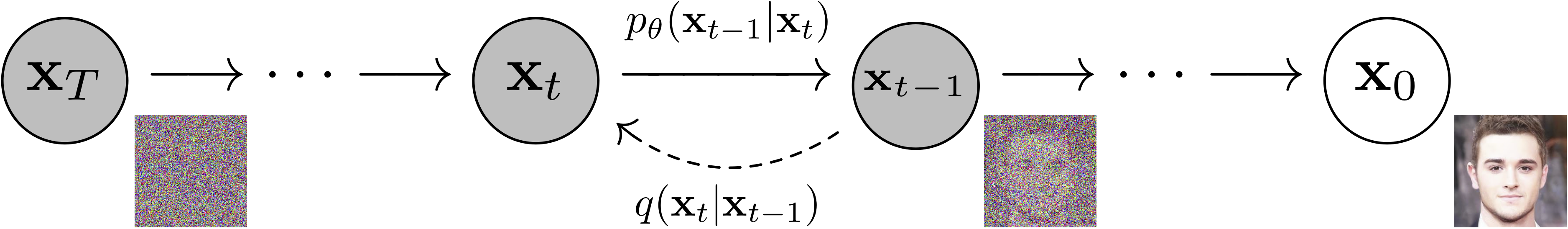
Diffusion models have recently gained popularity by obtaining exceptional high-quality image synthesis (and data likelihoods) while being easy to train. They, too, are latent variable models, but instead of encoding the data directly to a Gaussian random variable, the data is slowly diffused into one by adding many small noise variables. See the following figure (taken from Jonathan Ho’s post).
This post details how the models are formally developed and provide a simple implementation. Specifically, we follow the Kingma et al., 2021 paper titled Variational Diffusion Models.
Model Development
In a sense, a diffusion model can be seen as many Variational Autoencoders stacked on top of each other, and the encoders are fixed as linear Gaussians. In the continuous case, we assume infinitely many encoders. Every number from the interval $[0, 1]$ determines such an encoder as follows:
\[q(\mathbf z_t \mid \mathbf x)=\mathcal{N}(\alpha_t \mathbf x, \sigma_t^2 \mathbf I),\]where $\alpha_t$ and $\sigma_t$ make the (signal to) noise schedule. $\mathbf x$ is the data point, and $\mathbf z_t$ is the encoded variable. We also assume that the signal-to-noise ratio $\alpha_t^2 / \sigma_t^2$ decreases monotonically with $t$. As such, the encoding process is an additive Gaussian noise process. When $t$ is close to $0$, the image is hardly affected. When $t$ approaches $1$, we desire it to be close to a normal distribution. That is, all signal is diffused into Gaussian noise. In the following, however, we treat $t$ as a discrete variable going from $1$ to $T$. For the continuous case, see the Variational Diffusion Models paper. The process can be modeled with a Markov chain of many additive Gaussian noise transitions.
\[\mathbf x \rightarrow \dots \rightarrow \mathbf z_s \rightarrow \dots \rightarrow \mathbf z_{t-1} \rightarrow \mathbf z_t \rightarrow \mathbf z_{t+1} \rightarrow \dots \rightarrow \mathbf z_T\]Therefore, the inference distribution factorizes as
\[q(\mathbf z_{1:T}, \mathbf x) = q(\mathbf x) q(\mathbf z_1 \mid \mathbf x) \prod_{t=2}^T q(\mathbf z_t | \mathbf z_{t-1}).\]This is also called the forward process. We can analytically obtain $q(\mathbf z_t \mid \mathbf z_{t-1})$. We know that, by definition, $\mathbf z_{t-1} \sim \mathcal{N}(\alpha_{t-1} \mathbf x, \sigma_{t-1}^2 \mathbf I)$. Therefore, since the noise process is monotonic
\[\mathbf z_t \sim \mathcal{N}(\alpha_{t|t-1} \alpha_{t-1} \mathbf x,\, \alpha_{t|t-1}^2 \sigma^2_{t-1} \mathbf I + \sigma^2_{t|t-1}\mathbf I)\]Here, we used the fact that scaling a Gaussian random variable with a factor scales its variance with that factor squared (and included the assumed additive noise term with variance $\sigma_{t \mid t-1}^2$). We also know that $\mathbf z_t \sim \mathcal{N}(\alpha_t \mathbf x, \sigma_t^2 \mathbf I)$. Hence,
\[\alpha_{t|t-1} \alpha_{t-1} \mathbf x = \alpha_t \mathbf x \iff \alpha_{t|t-1} = \frac{\alpha_t}{\alpha_{t-1}}\] \[\alpha_{t|t-1}^2 \sigma^2_{t-1} \mathbf I + \sigma^2_{t|t-1} \mathbf I = \sigma^2_t \mathbf I \iff \sigma^2_{t|t-1} = \sigma^2_t - \alpha_{t|t-1}^2 \sigma^2_{t-1}\]Therefore, we see that
\[q(\mathbf z_t \mid \mathbf z_{t-1}) = \mathcal{N}(\alpha_{t|t-1} \mathbf z_{t-1}, \sigma_{t|t-1}^2\mathbf I)\]and we can directly compute the coefficients $\alpha_{t|t-1}$ and $\sigma_{t|t-1}$ from the known noise schedule parameters.
We have obtained a tractable inference distribution $q(\mathbf x, \mathbf z_{1:T})$. We now parameterize a model $p_\theta(\mathbf x, \mathbf z_{1:T})$ in the data generating direction (from noise to data). We minimize the relative entropy
\[\min D_{KL}[q(\mathbf x, \mathbf z_{1:T}) || p(\mathbf x, \mathbf z_{1:T})] = \min \mathbb{E}_{q(\mathbf x, \mathbf z_{1:T})} [\log q(\mathbf x, \mathbf z_{1:T}) - \log p(\mathbf x, \mathbf z_{1:T})]\]which we rewrite to
\[\min D_{KL}[q(\mathbf x, \mathbf z_{1:T}) || p(\mathbf x, \mathbf z_{1:T})] = \min \mathbb{E}_{q(\mathbf x)}\left[D_{KL}(q(\mathbf z_T \mid \mathbf x) || p(\mathbf z_T)) + \mathbb{E}_{q(\mathbf z_1 \mid \mathbf x)} [- \log p(\mathbf x \mid \mathbf z_1)] + \mathcal{L}_D\right] \tag{1},\]with
\[\mathcal{L}_D := \sum_{t=2}^T \mathbb{E}_{q(\mathbf z_t \mid \mathbf x)} \left[ D_{KL}[q(\mathbf z_{t-1} \mid \mathbf z_t, \mathbf x)||p(\mathbf z_{t-1} \mid \mathbf z_t)]\right] \tag{2}.\]We will discuss these terms in more detail later. Note that in $\mathcal{L}_D$, we replaced sampling through the Markov chain (ancestral sampling) with directly sampling $q(\mathbf z_t \mid \mathbf x)$.
\[\begin{aligned} \log q(\mathbf z_{1:T} | \mathbf x) - \log p(\mathbf z_{1:T}, \mathbf x) &= -\log p(\mathbf z_T)- \log p(\mathbf x \mid \mathbf z_1) + \log q(\mathbf z_1 \mid \mathbf x) + \sum_{t=2}^T \log q(\mathbf z_t|\mathbf z_{t-1}) - \log p(\mathbf z_{t-1}|\mathbf z_t) \\ &= -\log p(\mathbf z_T) - \log p(\mathbf x \mid \mathbf z_1) + \log q(\mathbf z_1 \mid \mathbf x) + \sum_{t=2}^T \log \left \{ q(\mathbf z_{t-1}|\mathbf z_t, \mathbf x) \cdot \frac{q(\mathbf z_t \mid \mathbf x)}{q(\mathbf z_{t-1} \mid \mathbf x)}\right \} - \log p(\mathbf z_{t-1}|\mathbf z_t) \\ &= -\log p(\mathbf z_T) - \log p(\mathbf x \mid \mathbf z_1) + \log q(\mathbf z_T \mid \mathbf x) + \sum_{t=2}^T \log q(\mathbf z_{t-1}|\mathbf z_t, \mathbf x) - \log p(\mathbf z_{t-1}|\mathbf z_t) \\ &= \log \frac{q(\mathbf z_T \mid \mathbf x)}{p(\mathbf z_T)} - \log p(\mathbf x \mid \mathbf z_1) + \sum_{t=2}^T \log \frac{q(\mathbf z_{t-1}|\mathbf z_t, \mathbf x)}{p(\mathbf z_{t-1}|\mathbf z_t)} \end{aligned}\]The second equality follows from Bayes’ rule:
\[q(\mathbf z_t \mid \mathbf z_{t-1}) \stackrel{\mathbf z_t \perp\!\!\perp \mathbf x \mid \mathbf z_{t-1}}{=} q(\mathbf z_t \mid \mathbf z_{t-1}, \mathbf x) = q(\mathbf z_{t-1} \mid \mathbf z_t, \mathbf x) \cdot \frac{q(\mathbf z_t \mid \mathbf x)}{q(\mathbf z_{t-1} \mid x)}.\]The follows from the many terms $q(\mathbf z_t \mid \mathbf x)$ and $q(\mathbf z_{t-1} \mid \mathbf x)$ cancel with each-other in the summation and with $q(\mathbf z_1 \mid \mathbf x)$ that was in front of it. Only $q(\mathbf z_T \mid \mathbf x)$ remains.
The obtained three terms form the loss function that we presented earlier.
Analyzing The Divergence
We study the terms of the objective function a bit more closely.
Diffusion Loss
Starting with the diffusion loss $\mathcal{L}_D$, we see that these can be rewritten so that we only have to perform data reconstruction during training.
\[\begin{aligned} q(\mathbf z_{t-1}\mid \mathbf z_t, \mathbf x) &= \frac{q(\mathbf z_t \mid \mathbf z_{t-1}, \mathbf x)}{q(\mathbf z_t \mid \mathbf x)} \cdot q(\mathbf z_{t-1} \mid \mathbf x) \\ &\stackrel{\mathbf z_t \perp\!\!\perp \mathbf x \mid \mathbf z_{t-1}}{=} \frac{q(\mathbf z_t \mid \mathbf z_{t-1})}{q(\mathbf z_t \mid \mathbf x)} \cdot q(\mathbf z_{t-1} \mid \mathbf x) \end{aligned}\]We already obtained an analytic form of the transition $q(\mathbf z_t \mid \mathbf z_{t-1})$ and we know $q(\mathbf z_{t-1} \mid \mathbf x)$ by construction. Since the transition is linear, $q(\mathbf z_t, \mathbf z_{t-1} \mid x)$ is jointly Gaussian. Therefore, using the well-known results for conditional Gaussians (e.g., Bishop (2006)) we get that
\[q(\mathbf z_{t-1} \mid \mathbf x, \mathbf z_t) = \mathcal{N}(\boldsymbol \mu_{t-1|t}, \sigma_{t-1|t}^2,\mathbf I),\]with
\[\begin{aligned} &\boldsymbol \mu_{t-1|t} = \frac{\alpha_{t|t-1}\sigma_{t-1}^2}{\sigma^2_t} \mathbf z_t + \frac{\alpha_{t-1} \sigma_{t|t-1}^2}{\sigma_t^2} \mathbf x,& \sigma_{t-1|t}^2 = \sigma_{t|t-1}^2 \frac{\sigma_{t-1}^2}{\sigma_t^2} \end{aligned}\]The reason why we performed all of these computations follows now. We have not parameterized $p(\mathbf z_{t-1} \mid \mathbf z_t)$ yet. If we parameterize it almost equivalently to $q(\mathbf z_{t-1} \mid \mathbf x, \mathbf z_t)$, then it turns out that we can simply perform a data reconstruction task at all times during training!
\[p_\theta(\mathbf z_{t-1} \mid \mathbf z_t) := q(\mathbf z_{t-1} \mid \mathbf z_t, \hat{\mathbf x}_\theta(\mathbf z_t; t))\]Since the KL-divergence between two Gaussianas involves a mean-squared error between the two means, we see that
\[D_{KL}\left[q(\mathbf z_{t-1}|\mathbf z_{t}, \mathbf x) || p_\theta(\mathbf z_{t-1}\mid \mathbf z_{t-1}) \right] \approx \Vert \boldsymbol \mu_{t-1|t} -\hat{\boldsymbol \mu}_{t-1|t}\Vert^2_2 = \left(\frac{\alpha_{t-1} \sigma_{t|t-1}^2}{\sigma_t^2}\right)^2 \Vert \mathbf x - \hat{\mathbf x}_\theta(\mathbf z_t; t) \Vert^2_2,\]where have omitted some terms involving the variances for conciseness (hence the “$\approx$”). As such, we are just reconstructing $\mathbf x$. For all details, consider the paper’s Appendix B Equations (34)-(40).
Furthermore, Since we know $\mathbf x$ and $\mathbf z_t$, our model can equivalently try to recover the additive noise through the relation:
\[\mathbf z_t = \alpha_t \mathbf x + \sigma_t \hat{\boldsymbol \epsilon}_\theta,\]which works better in practice.
Prior Loss
In eq. $(1)$ the first term is a prior loss, where $p(\mathbf z_T)$ is parameterized with a standard Gaussian. Since $q(\mathbf z_T \mid \mathbf x)$ is also Gaussian, we can compute the KL-divergence analytically.
Likelihood
The second term is a data likelihood term (e.g., reconstruction loss). We know that $\mathbf x$ has 256 distinct values.
We define a Gaussian \(r(\mathbf x \mid \mathbf z_1) := \mathcal{N}(\mathbf x \mid \hat{\mathbf x}_{\theta}(\mathbf z_1; 1), \sigma_1^2 \mathbf I)\) where $\hat{\mathbf x}_\theta(\mathbf z_1; 1)$ is the reconstructed image from the first time-step. As such, we re-use the same reconstruction network as in the diffusion loss. We can compute the likelihood analytically by integrating over the 256 possible values of $\mathbf x$.
\[\begin{aligned} p(\mathbf x \mid \mathbf z_1) &= \int_{\mathbf x - d_l}^{\mathbf x + d_u} r(\mathbf x \mid \mathbf z_1) d \mathbf x \\ &= \Phi((\mathbf x + d_u - \hat {\mathbf x}_\theta(\mathbf z_1; 1)) / \sigma_1) - \Phi((\mathbf x - d_u - \hat {\mathbf x}_\theta(\mathbf z_1; 1)) / \sigma_1) \end{aligned}\]Now, $d_u = d_l =0.5$ for $\mathbf x \in {1, \dots, 254}$, $d_l=\infty$ & $d_u = 0.5$ for $\mathbf x = 0$, and $d_u = \infty$ & $d_l = 0.5$ for $\mathbf x = 255$ divide the whole space into 256 parts that naturally add to 1.
Note: in practice, since $q(\mathbf z_1) \approx q(\mathbf x)$, i.e., there is such little noise added to obtain $\mathbf z_1$ from $\mathbf x$, this loss is often omitted, or we simply put $p(\mathbf x \mid \mathbf z_1) := \mathcal{N}(\mathbf x \mid \mathbf z_1, \sigma_1^2 \mathbf I)$.
Continuous Time
Note that we know $q(\mathbf z_t \mid \mathbf z_s)$ analytically for every $s$ < $t$, even when we use continuous-time $t \in [0, 1]$! This is shown analogously to how we showed it for $q(\mathbf z_t \mid \mathbf z_{t-1})$. Adding the fact that our diffusion loss simply reconstructs $\mathbf x$ (or equivalently, recover $\boldsymbol \epsilon$) means that we can sample $t$ from a continuous interval and keep performing the reconstruction task. We need to discretize only when we sample from the model (as shown later).
The diffusion loss, as shown in Appendix B.3., finally becomes
\[\mathcal{L}_D:= -\frac12 \mathbb{E}_{\boldsymbol \epsilon \sim \mathcal{N}(0, \mathbf I), t \sim U(0, 1)}\left[ \log\mathrm{SNR'}(t) \Vert \boldsymbol \epsilon - \hat{\boldsymbol \epsilon}_\theta(\mathbf z_t; t) \Vert^2_2 \right], \tag{3}\]with $\log\mathrm{SNR’}(t) = \frac{d \log \mathrm{SNR}(t)}{dt} = \frac{d \log \alpha_t^2 / \sigma_t^2}{dt}$.
This loss function is a continuous version approximation of $(2)$, using Monte Carlo integration.
Learned Noise Schedule
We left open the question how to set $\alpha_t$ and $\sigma_t$. So long as we stick to the requirements (monotonicity), we can learn the noise schedule. To do so, we implement a monotonic neural network that takes a time-step $t$ and outputs a (log) signal-to-noise ratio $\alpha_t^2 / \sigma_t^2$.
Implementation
We have all the required ingredients to start coding. For our full code, click here.
First we implement the “prior loss” part of $(3)$ (but now using continuous time, $t \in [0, 1]$). Note that gaussian_kl by default is against a zero mean Gaussian.
    def prior_loss(self, x, batch_size):
        logsnr_1, _ = self.snrnet(torch.ones((batch_size,), device=x.device))
        alpha_sq_1 = torch.sigmoid(logsnr_1)[:, None, None, None]
        sigmasq_1 = 1 - alpha_sq_1
        alpha_1 = alpha_sq_1.sqrt()
        mu_1 = alpha_1 * x
        return gaussian_kl(mu_1, sigmasq_1).sum() / batch_size
Next, the data likelihood. Since our $\mathbf x$ is scaled between $[-1, 1]$, we use $1 / 255$ instead of $0.5$ in the integration boundary. From $-1$ and $1$ we integrate to $-\infty$ and $\infty$, respectively. Since the CDF is 0 and $1$ for these ranges we can fill those values directly.
    def data_likelihood(self, x, batch_size):
        logsnr_0, _ = self.snrnet(torch.zeros((1,), device=x.device))
        alpha_sq_0 = torch.sigmoid(logsnr_0)[:, None, None, None].repeat(*x.shape)
        sigmasq_0 = 1 - alpha_sq_0
        alpha_0 = alpha_sq_0.sqrt()
        mu_0 = alpha_0 * x
        sigma_0 = sigmasq_0.sqrt()
        d = 1 / 255
        p_x_z0 = standard_cdf((x + d - mu_0) / sigma_0) - standard_cdf((x - d - mu_0) / sigma_0)
        p_x_z0[x == 1] = 1 - standard_cdf((x[x == 1] - d - mu_0[x == 1]) / sigma_0[x == 1])
        p_x_z0[x == -1] = standard_cdf((x[x == -1] + d - mu_0[x == -1]) / sigma_0[x == -1])
        nll = -torch.log(p_x_z0)
        return nll.sum() / batch_size
Third, we implement the most important part: the diffusion loss, along with the overall loss function $(3)$.
    def get_loss(self, x):

        batch_size = len(x)

        e = torch.randn_like(x)
        t = torch.rand((batch_size,), device=self.device)

        mu_zt_zs, sigma_zt_zs, norm_nlogsnr_t = self.q_zt_zs(zs=x, t=t)

        zt = mu_zt_zs + sigma_zt_zs * e

        e_hat = self.denoise_fn(zt.detach(), norm_nlogsnr_t)

        t.requires_grad_(True)
        logsnr_t, _ = self.snrnet(t)
        logsnr_t_grad = autograd.grad(logsnr_t.sum(), t)[0]

        diffusion_loss = (
            -0.5
            * logsnr_t_grad
            * F.mse_loss(e, e_hat, reduction="none").sum(dim=(1, 2, 3))
        )
        diffusion_loss = diffusion_loss.sum() / batch_size
        prior_loss = self.prior_loss(x, batch_size)
        data_loss = self.data_likelihood(x, batch_size)

        loss = diffusion_loss + prior_loss + data_loss

        return loss
We sample time-steps between $t \in [0, 1]$. Then, we sample from the diffusion process $q(\mathbf z_t|\mathbf z_s)$. Remember that, as we have shown above (“Model Development”), we can sample from these directly in terms of the parameters $\alpha_t$ and $\sigma_t$ and input $x$. We sample using reparameterization and reconstruct the noise using denoise_fn, which we will discuss later. Furthermore, in $(3)$ we see that we need a derivative of the log-signal-to-noise ratio. Since we implemented this schedule with a neural network, we compute it using autograd. Finally, we compute the diffusion loss. It’s multiplied with $-0.5$ since our SNR network is monotonically increasing instead of decreasing.
Now, let’s zoom in on q_zt_zs, the forward noising model.
    def q_zt_zs(self, zs, t, s=None):

        if s is None:
            s = torch.zeros_like(t)

        logsnr_t, norm_nlogsnr_t = self.snrnet(t)
        logsnr_s, norm_nlogsnr_s = self.snrnet(s)

        alpha_sq_t = torch.sigmoid(logsnr_t)
        alpha_sq_s = torch.sigmoid(logsnr_s)

        alpha_t = alpha_sq_t.sqrt()
        alpha_s = alpha_sq_s.sqrt()

        sigma_sq_t = 1 - alpha_sq_t
        sigma_sq_s = 1 - alpha_sq_s

        alpha_sq_tbars = alpha_sq_t / alpha_sq_s
        sigma_sq_tbars = sigma_sq_t - alpha_sq_tbars * sigma_sq_s

        alpha_tbars = alpha_t / alpha_s
        sigma_tbars = torch.sqrt(sigma_sq_tbars)

        return alpha_tbars * zs, sigma_tbars, norm_nlogsnr_t
Note that by putting $\alpha^2_t := \sigma(\gamma(t))$, where $\gamma$ is our learned SNR schedule, we keep $\alpha_t^2 + \sigma_t^2 = 1$.
\[\sigma\left(\log \frac{\alpha^2}{\sigma^2}\right) = \frac{1}{1+e^{\log \sigma^2 / \alpha^2}} = \frac{1}{1+\sigma^2 / \alpha^2} = \frac{\alpha^2}{\sigma^2 + \alpha^2} = \alpha^2\]This is fine, as the authors show that the continuous-time model is invariant to the noise schedule and, therefore, also the absolute values. Only the signal-to-noise ratios of the beginning and endpoints are essential.
Then, in the code, we use the formulas for $\alpha^2_{t\mid s}$ that we derived earlier and return the mean and standard deviation (and a normalized log-SNR for the denoising model to condition on).
That’s it! More is not needed for training. The implementations for the denoising model (a UNet-type) and the SNRnet are given later. We first zoom in on how to sample from the model.
Sampling
Sampling from a diffusion model is easy but requires much computation. We need to discretize the reverse diffusion process and iterate through the process.
\[\mathbf x \leftarrow \dots \leftarrow \mathbf z_{s} \leftarrow \dots \leftarrow \mathbf z_t \leftarrow \dots \leftarrow \mathbf z_T\]I.e., we sample $\mathbf z_t \sim p(\mathbf z_T)$ and use our learned $p(\mathbf z_{t-1} \mid \mathbf z_t)$ to iteratively sample until we reach $t=0$. We are free to choose the discretization granularity, but the paper shows that more time-steps is better.
    @torch.no_grad()
    def sample_loop(self, batch_size):


        img = torch.randn(shape, device=self.device)

        timesteps = torch.linspace(0, 1, self.num_timesteps)

        for i in tqdm(
            reversed(range(1, self.num_timesteps)),
            desc="Time-step",
            total=self.num_timesteps,
        ):

            t = torch.full((batch_size,), timesteps[i], device=img.device)
            s = torch.full((batch_size,), timesteps[i - 1], device=img.device)

            img = self.p_sample(img, t=t, s=s)
        return img
Here, we see that the number of time-steps is set by self.num_timesteps, and $[0, 1]$ is simply split into this number of parts.
    @torch.no_grad()
    def p_sample(self, x, t, s, clip_denoised=True, repeat_noise=False):
        b, *_, device = *x.shape, x.device

        model_mean, model_variance = self.p_mean_variance(
            zt=x, t=t, s=s, clip_denoised=clip_denoised
        )
        noise = noise_like(x.shape, device, repeat_noise)
        # no noise when s == 0
        nonzero_mask = (1 - (s == 0).float()).reshape(b, *((1,) * (len(x.shape) - 1)))
        return model_mean + nonzero_mask * model_variance.sqrt() * noise
Next, we implement $p(\mathbf z_s \mid \mathbf z_t)$.
    def p_zs_zt(self, zt, t, s, clip_denoised: bool):

        logsnr_t, norm_nlogsnr_t = self.snrnet(t)
        logsnr_s, norm_nlogsnr_s = self.snrnet(s)

        alpha_sq_t = torch.sigmoid(logsnr_t)[:, None, None, None]
        alpha_sq_s = torch.sigmoid(logsnr_s)[:, None, None, None]

        alpha_t = alpha_sq_t.sqrt()
        alpha_s = alpha_sq_s.sqrt()

        sigmasq_t = 1 - alpha_sq_t
        sigmasq_s = 1 - alpha_sq_s

        alpha_sq_tbars = alpha_sq_t / alpha_sq_s
        sigmasq_tbars = sigmasq_t - alpha_sq_tbars * sigmasq_s

        alpha_tbars = alpha_t / alpha_s
        sigma_tbars = torch.sqrt(sigmasq_tbars)

        sigma_t = sigmasq_t.sqrt()

        e_hat = self.denoise_fn(zt, norm_nlogsnr_t)

        if clip_denoised:
            e_hat.clamp_((zt - alpha_t) / sigma_t, (zt + alpha_t) / sigma_t)

        mu_zs_zt = (
            1 / alpha_tbars * zt - sigmasq_tbars / (alpha_tbars * sigma_t) * e_hat
        )
        sigmasq_zs_zt = sigmasq_tbars * (sigmasq_s / sigmasq_t)

        return mu_zs_zt, sigmasq_zs_zt
We know that
\[p(\mathbf z_s \mid \mathbf z_t) = q(\mathbf z_s \mid \mathbf z_t, \mathbf x=\hat{\mathbf x}_\theta(\mathbf z_t; t)).\]Our model outputs estimated noise and since $\mathbf z_t = \alpha_t \mathbf x + \sigma_t \boldsymbol \epsilon \iff \mathbf{x} = \frac{\mathbf z_t - \sigma_t \epsilon}{\alpha_t}$ we get (we shorthand $\hat{\mathbf x} := \hat{\mathbf x}_\theta(\mathbf z_t; t))$)
\[\begin{aligned} \hat{\mu}_{s \mid t} &= \frac{\alpha_{t\mid s} \sigma^2_s}{\sigma_t^2} \mathbf z_t + \frac{\alpha_s \sigma^2_{t\mid s}}{\sigma_t^2} \hat{\mathbf x} \\ &= \left( \frac{\alpha_{t\mid s} \sigma^2_s}{\sigma_t^2} + \frac{\alpha_s \sigma^2_{t\mid s}}{\alpha_t \sigma_t^2}\right)\mathbf z_t- \frac{\alpha_s \sigma^2_{t\mid s}}{\sigma_t^2}\frac{\sigma_t}{\alpha_t}\hat{\boldsymbol \epsilon} \\ &= \left( \frac{\alpha_{t\mid s} \sigma^2_s + \alpha_{t \mid s}^{-1} \sigma^2_{t\mid s}}{ \sigma_t^2} \right)\mathbf z_t- \alpha_{t|s}^{-1}\frac{\sigma^2_{t\mid s}}{\sigma_t}\hat{\boldsymbol \epsilon} \\ &= \left( \frac{\alpha_{t\mid s} \sigma^2_s + \alpha^{-1}_{t \mid s}(\sigma_t^2 - \alpha_{t\mid s}^2 \sigma_s^2)}{ \sigma_t^2} \right)\mathbf z_t- \frac{\sigma^2_{t\mid s}}{\alpha_{t|s}\sigma_t}\hat{\boldsymbol \epsilon} \\ &= \frac{1}{\alpha_{t \mid s}} \mathbf z_t- \frac{\sigma^2_{t\mid s}}{\alpha_{t|s}\sigma_t}\hat{\boldsymbol \epsilon} \\ \end{aligned}\]This final line is what we coded. The variance remains the same as $q(\mathbf z_s \mid \mathbf z_t, \mathbf x)$.
Finally, since $\mathbf x$ should be bounded between $[-1, 1]$, we know that $\hat{\boldsymbol \epsilon}$ should also be bounded as
\[\begin{aligned} &-1 \leq \mathbf x \leq 1\\ \iff &-1 \leq \frac{\mathbf z_t - \sigma_t \hat{\boldsymbol \epsilon}}{\alpha_t} \leq 1 \\ \iff &-\mathbf z_t -\alpha_t \leq - \sigma_t \hat{\boldsymbol \epsilon} \leq - \mathbf z_t + \alpha_t \\ \iff &\frac{\mathbf z_t - \alpha_t}{\sigma_t} \leq \hat{\boldsymbol \epsilon} \leq \frac{ \mathbf z_t + \alpha_t}{\sigma_t} \end{aligned}\]which is also coded in the provided snippet.
That concludes sampling!
Remaining Bits
Some final details are how the learned noise schedule is implemented and the specific model choices.
We do not strictly follow what the authors propose in our code but stick to the previous diffusion UNet-type architecture provided by the Lucidrains repository. The learned noise schedule (determined by the signal-to-noise ratios) is coded as follows (taken from the revsic repo).
class SNRNetwork(nn.Module):
    def __init__(self) -> None:
        super().__init__()

        self.l1 = PositiveLinear(1, 1)
        self.l2 = PositiveLinear(1, 1024)
        self.l3 = PositiveLinear(1024, 1)

        self.gamma_min = nn.Parameter(torch.tensor(-10.0))
        self.gamma_max = nn.Parameter(torch.tensor(20.0))

        self.softplus = nn.Softplus()

    def forward(self, t: torch.Tensor):  # type: ignore

        # Add start and endpoints 0 and 1.
        t = torch.cat([torch.tensor([0.0, 1.0], device=t.device), t])
        l1 = self.l1(t[:, None])
        l2 = torch.sigmoid(self.l2(l1))
        l3 = torch.squeeze(l1 + self.l3(l2), dim=-1)

        s0, s1, sched = l3[0], l3[1], l3[2:]

        norm_nlogsnr = (sched - s0) / (s1 - s0)

        nlogsnr = self.gamma_min + self.softplus(self.gamma_max) * norm_nlogsnr
        return -nlogsnr, norm_nlogsnr
with
class PositiveLinear(nn.Module):
    def __init__(self, in_features: int, out_features: int) -> None:
        super().__init__()

        self.weight = nn.Parameter(torch.randn(in_features, out_features))
        self.bias = nn.Parameter(torch.zeros(out_features))
        self.softplus = nn.Softplus()

    def forward(self, input: torch.Tensor):  # type: ignore
        return input @ self.softplus(self.weight) + self.softplus(self.bias)
Again, for all details, see our full implementation here.
Conclusion
Denoising diffusion models have many potential applications. It remains to be seen how long diffusion models will be around as the go-to generative model. Being easy to train, conceptually simple, and highly scalable, they certainly have valuable properties. But the relatively slow sampling procedure might be problematic. Despite this, I am optimistic. Please don’t hesitate to contact me if you have any questions or comments regarding the implementation, code, or diffusion models in general!