C2C 1: Complex and Quaternion Neural Networks
Introduction
Complex and quaternion numbers add depth to our numerical representations with their additional dimensions, enabling them to encapsulate more information more efficiently. By nature, they are better equipped to represent phenomena that involve both magnitude and phase (such as electromagnetic waves), or three-dimensional rotations.
This shift in perspective is not just a simple change in the data representation. It paves the way for more advanced neural network architectures. This post serves as a first step in a series that explores these, called Complex To Clifford (C2C). In upcoming works, we will explore Clifford algebras. As a natural extension of complex and quaternion numbers, Clifford algebra allows us to operate in multiple dimensions efficiently and opens the door to a collection of geometrically inspired deep learning models. Finally, we will culminate in the exploration of equivariant Clifford networks, which take advantage of these geometric insights to deliver impressive performance on a variety of tasks while maintaining certain equi- or invariances.
A selection of papers that explores (modern) (hyper)complex neural networks architecture is Danihelka et al. (ICML 2016), Trabelsi et al. (ICLR 2018), Parcollet et al. (ICLR 2019), Tay et al. (ACL 2019), Zhang et al. (ICLR 2021), Brandstetter et al. (ICLR 2023), Ruhe et al. (ICML 2023), Ruhe et al. (2023), and Brehmer et al. (2023). These works are largely incremental; hence, we discuss them in this series in chronological order. The posts in this series are:
- C2C 1: Complex and Quaternion Neural Networks
- C2C 2: Clifford Neural Layers for PDE Modeling
- C2C 3: Geometric Clifford Algebra Networks
- C2C 4: Clifford Group Equivariant Neural Networks
If you are unfamiliar with the Clifford algebra, I highly suggest studying these in order. If anything is unclear, please let me know in the comments below, or get in touch with me directly!
In this post, we focus on the following papers, which propose complex and quaternion-valued networks, respectively.
- Chiheb Trabelsi et al. (ICLR 2018): Deep Complex Networks
- Parcollet et al. (ICLR 2019): Quaternion Recurrent Neural Networks
Outline
- Why go complex? A short motivation for (hyper)complex neural networks.
- An introduction to complex numbers and quaternions. A quick recap on these fields.
- Complex neural networks. An introduction to how neural networks might be constructed using the complex field.
- Quaternion neural networks. Similar, but for the quaternions.
- Conclusion. A wrapup and preview of what’s coming up next in this series.
Why go complex?
Complex- and quaternion-valued neural networks offer several unique advantages compared to traditional real-valued neural networks. Here, we list a few of those.
- Richer Representations. Complex- and quaternion-valued neural networks can provide richer representations and transformations. For instance, complex numbers can naturally model phenomena characterized by both magnitude and phase, such as waves in physics, electrical signals, etc. Quaternion numbers, which extend complex numbers by adding two more imaginary parts, are highly effective in representing rotations in 3D space, which can be valuable for computer graphics, robotics, and more.
- Neuron Coupling. Similarly to the idea of Capsule Networks, incorporating complex or higher-order numbers in neural networks allow neurons to be coupled in a precise and meaningful way. In this sense, the neural network’s activations are not just values, but also contain directional information.
- Efficiency. The interplay within the neurons is fixed by the algebraic rules of (hyper)complex multiplication. By doing so, we get fully-connected layers without learning a full weight matrix. This can yield significant savings in memory and computational costs.
An introduction to complex numbers and quaternions.
Naturally, please skip ahead if a quick refresh on these numbers is not needed.
Complex Numbers
Complex numbers extend the concept of the one-dimensional number line to two dimensions. A complex number can be defined using two real numbers: the real part and the imaginary part. The set of all complex numbers is denoted by the symbol $\mathbb{C}$.
A complex number is typically written as $z = a + bi$ where $a$ and $b$ are real numbers, and $i$ is the imaginary unit with the property $i^2 = -1$.
Operations with complex numbers are defined in terms of operations with real numbers. Addition and multiplication are defined as follows:
- Addition: $(a + bi) + (c + di) = (a + c) + (b + d)i$
- Multiplication: $(a + bi)(c + di) = ac - bd + (bc + ad)i$
Note that the multiplication formula results from applying the distributive law and using the fact that $i^2 = -1$.
A well-known application of complex numbers can be found in Fourier analysis, where a signal can be decomposed into sums of trigonometric functions, which can be represented using complex exponentials representing amplitudes and phases.
Quaternions
Quaternions extend the idea of complex numbers into four dimensions. They are typically denoted by the symbol $\mathbb{H}$. A quaternion number is generally represented as $q = a + bi + cj + dk$, where $a, b, c$, and $d$ are real numbers, and $i, j$, and $k$ are the quaternion units. They follow the rules: $i^2 = j^2 = k^2 = ijk = -1$.
Adding quaternions, similarly to complex numbers, goes component-wise. Multiplication of quaternions, however, is non-commutative; that is, the order of the factors changes the result. The product of two quaternions $p = a + bi + cj + dk$ and $q = e + fi + gj + hk$ is given by:
\[\begin{aligned} pq &= ae - bf - cg - dh \\ &+ (af + be + ch - dg)i \\&+ (ag - bh + ce + df)j \\&+ (ah + bg - cf + de)k \end{aligned}\]The most famous application of quaternions is that they can be used to represent rotations in three dimensions more effectively and intuitively than other methods, such as rotation matrices or Euler angles.
Hamilton’s crucial discovery to model three-dimensional rotations was not to extend complex numbers to three but to four dimensions. During this flash of inspiration, he was walking along the Royal Canal in Dublin, and immediately carved the basic quaternion equations into the side of Brougham Bridge.
Complex Neural Networks
First, I’d like to start with a note on training complex neural networks. Generally, the papers we discuss here apply backpropagation in its native form (i.e., by using PyTorch’s automatic differentiation) and do not consider specialized complex or quaternion derivatives.
Here, we follow Trabelsi et al., Deep Complex Networks. The main idea is simply to replace any real-valued multiplication - as done in regular neural networks - with a complex-valued one. To do so, one first needs to represent the complex field in a PyTorch tensor data structure. Since complex numbers have real and imaginary components, we can construct a weight matrix $W \in \mathbb{R}^{c_{\mathrm{out}} \times c_{\mathrm{in}} \times 2}$, which can be interpreted as $W \in \mathbb{C}^{c_{\mathrm{out}} \times c_{\mathrm{in}}}$. If we now have a complex feature vector $h \in \mathbb{R}^{c_{\mathrm{in}} \times 2}$, then complex matrix multiplication follows
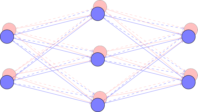
\[Wh = Ax - By + i (Bx + Ay),\]where we use $A := \Re(W)$, $x:= \Re(h)$, $y:=\Im(h)$, and $B:=\Im(W)$. Trabelsi et al. further extend this to complex convolutions, but the idea remains the same. We see how we automatically get full mixing between the real and imaginary parts governed by the same parameters $A$ and $B$. This is also illustrated in the header figure at the top of this post. We will discuss this parameter sharing in more detail below.
Activation Functions and Normalization
The proposed activation simply applies a ReLU unit independently to the real and imaginary parts. This means that for $h \in \mathbb{R}^{c_{\mathrm{in}} \times 2}$ we can simply apply $h \mapsto \mathrm{ReLU}(h)$ in PyTorch. Regarding backpropagation, this function is not strictly holomorphic, i.e., complex diffentiable everywhere. However, we can still apply the backpropagation algorithm by considering the coefficients of the complex numbers as independent real numbers.
Let’s now consider batch normalization. Batch normalization is a common technique in deep learning that uses batch statistics to renormalize the values of a hidden representation to a well-behaved range. To do so, one computes batch-wide mean and variance statistics. Since we now work with complex-valued representations containing both a real and an imaginary part, we can consider a covariance statistic. As such, we can put
\[h \mapsto (V)^{-\frac 12}(h - \mathbb{E}[h]),\]where the covariance and expectation are empirically estimated using the minibatch. We have
\[V:=\begin{pmatrix} V_{rr} & V_{ri} \\ V_{ir} & V_{ii} \end{pmatrix} = \begin{pmatrix} \mathrm{Cov}\left( \Re(h), \Re(h) \right) & \mathrm{Cov}\left( \Re(h), \Im(h) \right) \\ \mathrm{Cov}\left(\Im(h), \Re(h) \right) & \mathrm{Cov}\left( \Im(h), \Im(h) \right) \end{pmatrix}.\]Note that this covariance matrix becomes rather expensive when the number of components per element grows. For example, for quaternions, this would already become a $4 \times 4$ matrix. For even higher-dimensional fields, this will become unattainable.
Implementation
Presently, PyTorch natively supports many complex-valued operations by simply casting your data to the torch.cfloat format.
We present an example of a complex linear layer and the component-wise ReLU below.
For the batch normalization as discussed above consult, for example, this page.
import torch
from torch import nn
import torch.nn.functional as F

linear = nn.Linear(64, 32).to(torch.cfloat)

x = torch.randn(8, 64, dtype=torch.cfloat)
x = linear(x)
x = x.real.relu() + 1j * x.imag.relu()
Experiment: MusicNet
Complex valued networks inherently posess several advantageous characteristics. First, there is a geometric component, since complex multiplication essentially computes a two-dimensional rotation. That means that if one has a dataset containing two-dimensional vector-valued information, this can effectively be represented as a complex number. I.e., instead of operating in the two-dimensional Euclidian plane, we operate in the complex plane. Second, complex-valued networks can incorporate information regarding the phase of a signal through the imaginary part. This is why they have achieved state-of-the-art performance in several audio related tasks, where the data have wave characteristics. Further, applying Fourier analysis to this data during preprocessing would readily present complex-valued inputs to the network. Complex neural networks will respect the nature of such data.
In this paper, the authors focus on the latter case. We focus on their music transcription experiment. Given the waveform, the models’ task is to predict which notes (out of 84) are being played. Since multiple notes can be played at the same time, the output distributions are given by 84 independent sigmoid units. Having access to a model that can effectively perform this task can have a significant impact for musicians, music teachers, and many other professionals in the music industry. It could considerably speed up the process of studying and sharing music. The results can be observed in the table below.
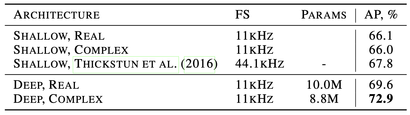
We see that the average precision (a classification-threshold independent precision metric) for the complex network is higher despite fewer trainable parameters!
Quaternion Networks
Using complex neural networks, we took a leap from the line (real numbers) to the plane (complex numbers). Several works have gone even further to introduce four-dimensional quaternion-valued networks. Here, we follow Parcollet et al., Quaternion Recurrent Neural Networks. The authors mainly motivate quaternion networks in analogy to Capsule Networks, that is, as a means to couple multidimensional data. Further, the Hamilton product between $h, w \in \mathbb{H}$, where $w$ are tunable weights, can be written in matrix form as
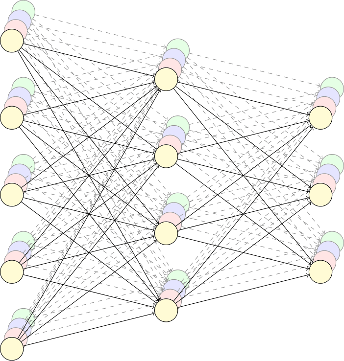
\[wx = \begin{bmatrix} w_0 & -w_1 & -w_2 & -w_3 \\ w_1 & w_0 & -w_3 & w_2 \\ w_2 & w_3 & w_0 & -w_1 \\ w_3 & -w_2 & w_1 & w_0 \end{bmatrix} \begin{bmatrix} x_0 \\ x_1 \\ x_2 \\ x_3 \end{bmatrix},\]where the indices indicate the coefficients of the real and $i, j, k$ parts of the quaternions. As such, where a fully connected layer would transform four values using 16 weights, we obtain weight sharing through quaternion multiplication by reusing the same four parameters using the Hamilton product. This can induce significant memory savings. Further, this weight sharing has meaning, as quaternions are used to compute spatial rotations.
Linear Layers
Similarly to the complex version, we now construct neural network linear layers by applying quaternion multiplication for every input and output channel. Let $h^{\mathrm{in}} \in \mathbb{R}^{c_{\mathrm{in}} \times 4}$ and $W \in \mathbb{R}^{c_{\mathrm{in}} \times c_{\text{out}} \times 4}$. Then a linear layer amounts to
\[h^{\text{out}}_{j} := \sum_{i = 1}^{c_{\text{in}}} W_{ij} h^{\text{in}}_{i} \,,\]where we use quaternion multiplication to compute $W_{ij} h_{i}$.
The code is now a bit more involved, as quaternion multiplication is not natively supported by PyTorch. One can effectively compute this using the following code, which is taken from the official implementation.
As one sees, we can use the weight matrix $W \in \mathbb{R}^{c_{\mathrm{in}} \times c_{\text{out}} \times 4}$ to obtain a quaternion weight matrix $W^{\text{quat}} \in \mathbb{R}^{4 c_{\mathrm{in}} \times 4 c_{\text{out}}}$ that directly carries out the linear Hamilton-product transformation (note the similarities to the matrix-form of the Hamilton product introduced earlier!). Since the Hamilton product is a linear transformation, and also the linear layer (obviously), it is clear that their combination can be expressed as a matrix multiplication.
Note that convolutional kernels can be constructed in similar manners.
The authors then continue to construct RNNs or even LSTMs from these layers, which follow similar principles to how traditional RNNs from linear layers using weight sharing through time.
Activations
Regarding activations, we can again apply component-wise ReLUs, similarly to the complex-valued networks. That is,
\[a(q) = f(h_0) + f(h_1)i + f(h_2)j + f(h_3)k \,,\]where $f$ is a ReLU (or any scalar activation function, for that matter).
Experiment: TIMIT Automatic Speech Recognition
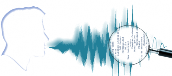
Quaternions can be interpreted as pairs of complex numbers. Hence, their application to audio data again makes sense for similar reasons as presented in the complex neural network section. The authors compare quaternion RNNs (QRNNs) against their usual counterparts on the TIMIT dataset. The performance measure is Phoneme Error Rate (PER): a measure often used in the field of speech recognition to evaluate the performance of a system. It represents the percentage of mistakes a system makes when trying to recognize individual phonemes - the smallest distinct units of sound in a particular language that differentiate one word from another.
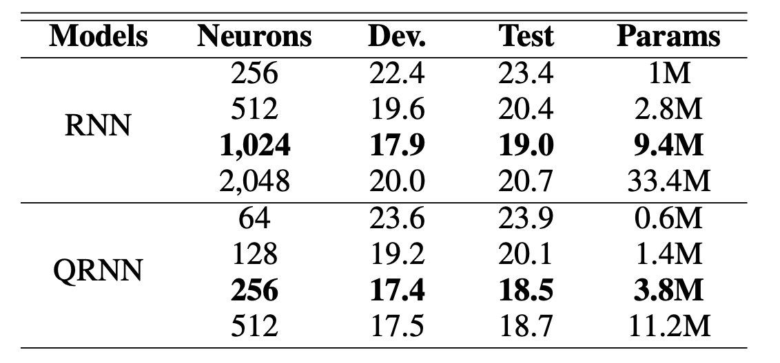
In the table, we see that QRNN was able to outperform the baseline (i.e., lower development (validation) and test error rates) given a much smaller parameter and neuron budget. This effective weight sharing can enable high-quality speech recognition on low computational devices like smartphones, which have restricted memory and processing power.
Conclusion
We’ve discussed how complex-valued networks open up new possibilities for richer data representations, using the power of the complex plane and the interaction between its real and imaginary components. We then dived into the four-dimensional space of quaternion-valued networks, witnessing how they can elegantly model multidimensional data and perform complex transformations with weight sharing, significantly reducing memory requirements. We’ve seen in various experiments, including two we’ve closely examined, that these networks offer distinct advantages and pave the way for new opportunities in the field of data science.
In the upcoming post, we will discuss how Clifford algebras can be used to obtain and generalize properties identical to the complex and quaternion networks discussed here. Because of this generalization, we can also go a step further with them and truly encode some geometry into neural networks. Let me know in the comments below if you have questions, comments, or ideas worth sharing!
Acknowledgments
I would like to thank Johannes Brandstetter, Jayesh Gupta, Marco Federici, and Jim Boelrijk for providing valuable feedback regarding this blogpost series.