C2C 2: Clifford Neural Layers for PDE Modeling
In the previous post of this series, we motivated and introduced complex and quaternion neural networks. Here, we discuss a recent paper that extends to Clifford algebras, obtaining further geometric inductive biases, which we will elaborate on.
A selection of papers that explores (modern) (hyper)complex neural networks architecture is Danihelka et al. (ICML 2016), Trabelsi et al. (ICLR 2018), Parcollet et al. (ICLR 2019), Tay et al. (ACL 2019), Zhang et al. (ICLR 2021), Brandstetter et al. (ICLR 2023), Ruhe et al. (ICML 2023), Ruhe et al. (2023), and Brehmer et al. (2023). These works are largely incremental; hence, we discuss them in this series in chronological order. The posts in this series are:
- C2C 1: Complex and Quaternion Neural Networks
- C2C 2: Clifford Neural Layers for PDE Modeling
- C2C 3: Geometric Clifford Algebra Networks
- C2C 4: Clifford Group Equivariant Neural Networks
If you are unfamiliar with the Clifford algebra, I highly suggest studying these in order. If anything is unclear, please let me know in the comments below, or get in touch with me directly!
In this post, we focus on the following work, which presents Clifford-valued neural layers and their applications to partial differential equation neural surrogates.
Outline
- The Clifford algebra. What are Clifford algebras?
- Clifford Neural Layers. How to construct Clifford neural layers?
- The Geometric Product. The fundamental algebra product.
- Experiment: the Navier-Stokes Equations. Modeling the Navier-Stokes equations using Clifford networks.
- Conclusion. A wrapup and preview of what’s coming up next in this series.
The Clifford Algebra
Let’s first start with a bit of history to place things in context. The Clifford algebra was introduced by William Kingdon Clifford in the late 19th century. As a mathematician, he was well-acquainted with Hamilton’s quaternions. At the same time, he was studying algebras over fields that were getting popular at that point, such as Grassman’s exterior algebra. After its identification, Clifford noted that his algebra possesses properties that complex numbers and quaternions also do, entirely from a geometric perspective.
Over time, this algebra has been incorporated into various branches of mathematics and physics. With the advent of the theory of relativity and quantum mechanics in the 20th century, Clifford algebra gained significance as a useful tool for encoding physical information. For instance, in the realm of quantum mechanics, Clifford algebra provides a natural language for Pauli and Dirac matrices, integral to quantum spin and the behavior of elementary particles. In the late 20th and early 21st centuries, Clifford algebra has also seen developments in computer science and robotics, assisting in representing and computing 3D rotations and other geometric transformations.
It is sometimes noted that Clifford himself referred to his algebra as the geometric algebra. This convention was also popularized by David Hestenes’ work on using geometric algebra for physics. Modern geometers that use the algebra on a daily basis like to distinguish its application to (computational) geometry from its mathematical properties by using geometric rather than Clifford algebra. Bottom line is: essentially, they are the same. These naming conventions unfortunately lead to much confusion; the papers listed above also use both naming conventions.
The quadratic form
The construction (apart from mathematical details) of the Clifford algebra is relatively simple. We take a regular vector space $V$ over a field $\mathbb{F}$ (usually the reals $\mathbb{R}$) and turn it into a quadratic vector space (denoted with a tuple $(V, Q)$) by endowing it with a quadratic form $Q$. This quadratic form $Q: V \to \mathbb{F}$ takes a vector and returns a scalar. We now say that for any vector $v \in V$, we have $v^2 = Q(v)$. That is, we assume we can multiply vectors, and relate it to the geometry of the vector space through its quadratic form. We will not go into more detail here, and the act of multiplying vectors will, later on, be elaborated on.
Regarding the quadratic form, we could write in matrix notation
\[v \mapsto Q(v) := v^\top G v.\]Here, $G$ is the metric, a (diagonal) matrix that is usually canonicalized to contain only entries of $1$ and $-1$. This means that we have basis vectors that square to either $1$ or $-1$. The arising Clifford algebra over the reals can be denoted as $\Cl_{p, q}(\Rbb)$. Here, $p$ and $q$ denote the number of basis vectors that square to $1$ and $-1$, respectively. Therefore, $\dim V = p + q$. More explicitly, we have for basis vector $e_i$:
\[\begin{aligned} \begin{cases} e_i^2 = Q(e_i) = 1 \qquad &1 \le i \le p \,, \\ e_i^2 = Q(e_i) = -1 \qquad &p < i \le p + q \,. \end{cases} \end{aligned}\]For example, consider $\Cl_{0, 2}(\mathbb{R})$, which has two basis vectors ($\dim \mathbb{R}^2 = 2$). Let’s examine the first one: $e_1$.
\[Q(e_1) = [1, 0]^\top \begin{bmatrix} -1 & 0 \\ 0 & -1 \end{bmatrix} [1, 0] = -1\]The Geometric Product
Let’s consider two vectors $a$ and $b$ expressed in the basis $\{e_1, e_2\}$. That is, we have a two-dimensional vector space, and we further assume that the metric is positive definite. In other words, we work in $\Cl_{2, 0}(\Rbb)$. Their geometric product looks as follows:
\[\begin{aligned} ab = (a_1 e_1 + a_2 e_2)(b_1 e_1 + b_2 e_2) &= a_1e_1(b_1 e_1 + b_2 e_2) + a_2 e_2 (b_1 e_1 + b_2 e_2) \\ &= a_1 b_1 e_1^2 + a_1 b_2 e_1 e_2 + a_2 b_1 e_2 e_1 + a_2 b_2 e_2^2 \\ &= (a_1 b_1 + a_2 b_2)1 + (a_1 b_2 - a_2 b_1)e_1 e_2 \,. \end{aligned}\]Let’s digest what happened here. In the first and second equations, we use the distributive property of the product, as well as the communicativity of scalar multiplication ($a, b \in \Rbb$). Then, we realize that $e_1$ and $e_2$ both square to $1$. Regarding the last line, we first take a slight detour and introduce the Clifford algebra basis.
The Clifford Algebra basis
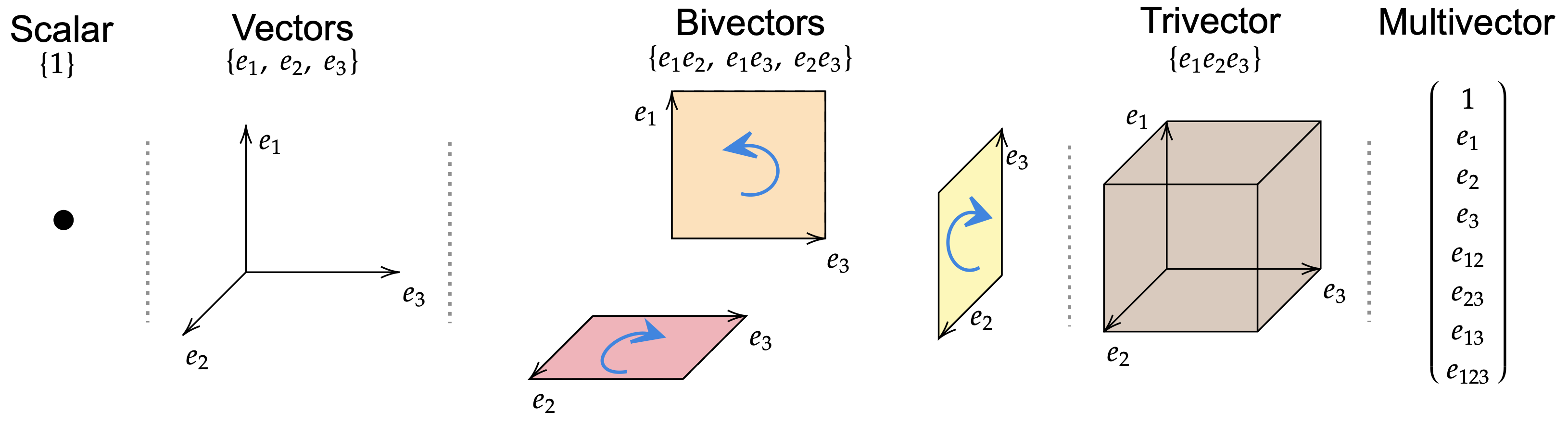
One can show that it is possible to construct a well-defined basis for the Clifford algebra. Further, this basis contains $2^n$ elements, where $n:= \dim V$. Regarding the $\Cl_{2, 0}(\Rbb)$ case, a general element $x$ can be written as
\[x = x_0 1 + x_1 e_1 + x_2 e_2 + x_{12} e_{12} \,.\]We see that it contains scalar elements (multiples of $1$) in $\Rbb$, and we naturally have vector elements in $V$. However, since we are allowed to take products, we can also produce $e_1 e_2$. This element cannot be reduced and is regarded as a valid basis element of the algebra. For $\Cl_{2, 0}(\Rbb)$, the basis therefore has $\{1, e_1, e_2, e_{12} \}$ ($e_{12} := e_1 e_2$), containing $4 = 2^2$ elements. $e_{12}$ being a product of two basis vectors is a bivector element. Geometrically, it represents an area-related quantity.
In three dimensions, we get
\[\{1, e_1, e_2, e_3, e_{12}, e_{13}, e_{23}, e_{123} \}\]which has $2^3=8$ elements. Here, we even get a trivector element, which relates to a volumetric quantity. Basis elements are also referred to as (basis) blades.
The bilinear form
Now, to completely understand how the final line of the geometric product derivation was obtained, we have to introduce the algebra’s bilinear form. The bilinear form $\langle \cdot, \cdot \rangle: V \times V \to \mathbb{F}$ is a function that is induced by the quadratic form. It takes two vectors and outputs a scalar. Using matrix notation, one can write
\[v_1, v_2 \mapsto \langle v_1, v_2 \rangle := v_1^\top G v_2\]Hence, when the vectors are equal, it reduces exactly to the quadratic form. When the metric is positive definite, it is exactly the dot product.
This bilinear form comes together with the fundamental Clifford identity (see, e.g., Wikipedia for details)
\[v_1 v_2 + v_2 v_1 = 2 \langle v_1, v_2 \rangle \,.\]Now, one can check that for orthogonal vectors (such as basis vectors), the bilinear form is $0$ (similar to taking dot products of orthogonal vectors). In those cases, we have the anticommutativity relation
\[e_1 e_2 = -e_2 e_1 \,.\]This is an extremely useful identity ensuring that we can always flip the order of basis vectors such that they end up in the arrangement that we constructed the algebra basis with. In the geometric product derivation, this is used in the final line to express the result $a_2 b_1 e_2 e_1$ into $-a_2 b_1 e_1 e_2$ and group it with the other $e_{12}$ element. You should now be able to re-derive the geometric product of two vectors 🙂.
The wedge product
Note that the scalar part of the geometric product (e.g., using the one we calculated above, the “$a_1 b_1 + a_2 b_2$” part) is equal to the bilinear form $\langle a, b \rangle$. Using the fundamental Clifford identity, we have that $\langle a, b \rangle = \frac 12 (ab + ba)$. In turn, this means that
\[ab = \frac12 (ab + ba) + \frac12(ab - ba)\]where the first term is the bilinear form, and the second term is added to retain equality. This term corresponds to the bivector part of the geometric product and is also known as the anticommutator or wedge product
\[a \wedge b := \frac 12 (ab - ba)\]which has similar properties to the wedge product from the exterior algebra. One can check that this results in the bivector part of our explicit computation of the geometric product.
As such, the geometric product of two vectors can be written as the sum of the dot product and wedge product
\[\Large ab = \langle a, b \rangle + a \wedge b\]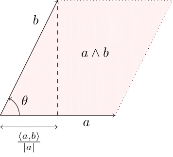
The product of two multivectors
We have investigated how one multiplies two vectors in the Clifford algebra. Using the algebra basis we identified, the product of two general elements (multivectors) $a$ and $b$ can be written as
\[(a_0 + a_1 e_1 + a_2 e_2 + a_{12}e_{12})(b_0 + b_1 e_1 + b_2 e_2 + b_{12} e_{12}).\]One can work out the result of this product using the same associativity, distributivity, and Clifford algebra rules as used above. In the source paper, one can find the entire derivation.
In matrix form, the new coefficients can be computed as
\[\begin{bmatrix} a_0 & g_1 a_1& g_2 a_2& -g_1 g_2 a_{12} \\ a_1& a_0& g_2 a_{12}& -g_2 a_2 \\ a_2& -g_1 a_{12}& a_0& g_1 a_1 \\ a_{12}& -a_2& a_1& a_0 \end{bmatrix} \begin{bmatrix} b_0 \\ b_1 \\ b_2 \\ b_{12}\end{bmatrix} \,.\]Here, $(g_1, g_2):= \mathrm{diag} \,G$. The resulting vector gives you the coefficients for the new scalar, vector, and bivector parts. Note the similarities to quaternion multiplication! In $\Cl_{0, 2}(\mathbb{R})$, we have $g_1 = g_2 = -1$. Plugging this in exactly gives the matrix form of the Hamilton product. More on this in the next section.
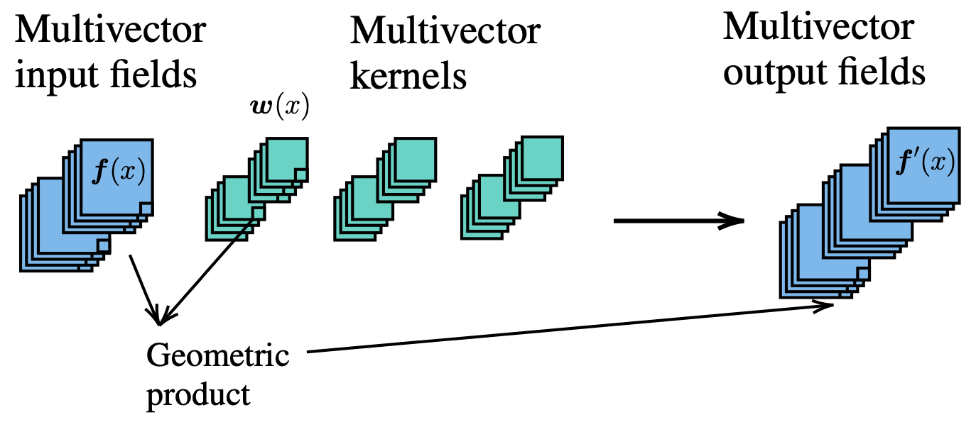
Clifford Neural Layers
Let’s now investigate how to construct Clifford layers! But first, the authors of the paper also propose a Clifford Fourier layer, which was inspired by the Fourier Neural Operator architecture, but can explicitly deal with vector-valued data. We will not discuss this layer in this post, and instead focus on a more natural continuation from the complex and quaternion-valued layers.
Let’s investigate the Clifford algebra $\Cl_{0, 1}(\Rbb)$. Its basis components are $\{1, e_1\}$, where $e_1^2=-1$. What does this remind us of? Exactly! The complex numbers $\Cbb$. That is, a multivector $a \in \Cl_{0,1}(\mathbb{R})$ behaves in many ways exactly the same as a complex number. For example, the geometric product in this algebra exactly computes complex multiplication.
Next, take $\Cl_{0, 2}(\Rbb)$. Here, we have ${1, e_1, e_2, e_{12}}$, with $e_1^2=e_2^2=e_{12}=-1$ and $e_1 e_2 e_{12} = - e_1^2 e_2^2 = -1$. These are exactly Hamilton’s quaternion relations! In this case, the geometric product computes the Hamilton product, i.e., quaternion multiplication.
Now we know that using the Clifford perspective, we can generalize the networks that we discussed in the previous post. Consider the following Python code taken from the official implementation.
def get_2d_clifford_kernel(
    w: Union[tuple, list, torch.Tensor, nn.Parameter, nn.ParameterList], g: torch.Tensor
) -> Tuple[int, torch.Tensor]:
    """Clifford kernel for 2d Clifford algebras, g = [-1, -1] corresponds to a quaternion kernel.

    Args:
        w (Union[tuple, list, torch.Tensor, nn.Parameter, nn.ParameterList]): Weight input of shape `(4, d~input~, d~output~, ...)`.
        g (torch.Tensor): Signature of Clifford algebra.

    Raises:
        ValueError: Wrong encoding/decoding options provided.

    Returns:
        (Tuple[int, torch.Tensor]): Number of output blades, weight output of shape `(d~output~ * 4, d~input~ * 4, ...)`.
    """
    assert isinstance(g, torch.Tensor)
    assert g.numel() == 2
    w = _w_assert(w)
    assert len(w) == 4

    k0 = torch.cat([w[0], g[0] * w[1], g[1] * w[2], -g[0] * g[1] * w[3]], dim=1)
    k1 = torch.cat([w[1], w[0], -g[1] * w[3], g[1] * w[2]], dim=1)
    k2 = torch.cat([w[2], g[0] * w[3], w[0], -g[0] * w[1]], dim=1)
    k3 = torch.cat([w[3], w[2], -w[1], w[0]], dim=1)
    k = torch.cat([k0, k1, k2, k3], dim=0)
    return 4, k
There are a few discrepancies with the quaternion kernel of the previous post and also with the matrix form of the Clifford product. Firstly, this kernel computes right multiplication with the weights. Second, this computes a convolutional kernel, which slightly permutes the order of some quantities. Further, the vital difference is that this kernel takes the metric $G$ as input (specifically, its diagonal). For $g=[-1, -1]$, we get the quaternion (right) multiplication kernel, as discussed above. For $g=[1, 1]$ we get the kernel for $\Cl_{2, 0}(\Rbb)$.
Using this kernel we can compute Clifford linear layers (or convolutions) with
\[h_{j}^{\text{out}} := \sum_{i=1}^{c_{\mathrm{in}}} W_{ij} h_i^{\text{in}}\]where $W_{ij} h_i$ denotes the geometric product (both are elements of $\Cl_{2, 0}(\Rbb)$). Again, since the geometric product is linear, we can reshape this (as done in the code) into a big weight matrix $W^{\text{geom}} \in \mathbb{R}^{2^n \cdot c_{\text{in}} \times 2^n \cdot c_{\text{out}}}$, where $2^n$ the dimension of the algebra.
Clifford rotational layers
As we saw above, the geometric product can naturally be geometrically interpreted. However, to obtain valid geometric transformations, one usually needs to focus on a specific set of geometric products. The authors additionally introduce Clifford rotational kernels, using an isomorphism from $\Cl_{0, 2}(\mathbb{R})$ to the quaternions $\mathbb{H}$. Quaternions can be used to compute three-dimensional rotations. As such, the authors propose a rotational kernel $R$, computed from a Clifford element. Specifically, we have
\[h_{j}^{\text{out}} := \sum_{i=1}^{c_{\mathrm{in}}} \underbrace{R(W_{ij}) [h_i^{\text{in}}]_{1, 2, 3}}_{\text{Matrix Multiplication}} + \underbrace{[W_{ij} h_i^{\text{in}}]_{0}}_{\text{Geometric Product}}.\]Let’s analyze this equation. Again, we are computing a linear combination of some products analogously to the complex, quaternion, and Clifford layers above. The first term, however, does not plainly apply $W_{ij}$. It first computes the rotational kernel from $W_{ij}$, denoted $R(W_{ij})$, which is a $3 \times 3$ matrix. It then gets applied to the two vector components and single bivector part of $h_i^{\text{in}}$, denoted $[h_i^{\text{in}}]_{1, 2, 3}$. This means that the scalar part of $h_i^{\text{in}}$ does not get transformed. Hence, we apply the geometric product for that part but consider only its scalar output.
This entire operation is still linear. However, empirically, the authors note that this rotational layer typically outperforms its Clifford layer counterpart. They hypothesize that this is due to the fact that rotation is a highly interpretable and valid geometric operation, where geometric products can be harder to interpret when applied to full multivectors. This will be further explored in the next blog post of this series.
For a code implementation of this kernel, see this page.
Activation and normalization
The authors follow the complex and quaternion networks regarding activation functions. That is, they apply component-wise ReLUs:
\[h \mapsto \text{CliffordReLU}(h) := \text{ReLU}([h_{i}]_0) + \text{ReLU}([h_{i}]_1)e_1 + \text{ReLU}([h_{i}]_2)e_2 + \text{ReLU}([h_{i}]_{12}) e_{12}.\]The batch normalization from the complex neural networks of Trabelsi et al. (see previous post) gets extended to a Clifford batch normalization:
\[h \mapsto (V)^{-\frac 12}(h - \mathbb{E}[h]),\]where the covariance matrix is now computed over all Clifford components. Note that since the algebra grows like $2^n$, this is generally rather expensive, and already computing a $4 \times 4$ covariance matrix (for an algebra over a two-dimensional vector space) for every neuron in your network proved to be slightly prohibitive.
Experiment: the Navier-Stokes equations
The paper focuses on applying their layers to obtain solutions to partial differential equations (PDEs). Partial differential equations, similar to ordinary differential equations (ODEs), describe the dynamics of a system through partial derivatives. They are the workhorses of many sciences. Obtaining a solution requires integrating the differential equations over time. Usually, however, a closed-form solution is elusive. To this end, scientists apply numerical integrations, such as Runge-Kutta schemes. For sufficiently hard problems (such as the Navier-Stokes equations), these are incredibly expensive to compute because they only yield faithful solutions when, e.g., the integration step $\Delta t$ is small enough. Machine learning and neural networks provide a promising tool for obtaining faithful solutions using a larger $\Delta t$.
The incompressible Navier-Stokes equations describe how a fluid behaves in a closed system. This behavior is highly nonlinear, making this a challenging problem to solve.
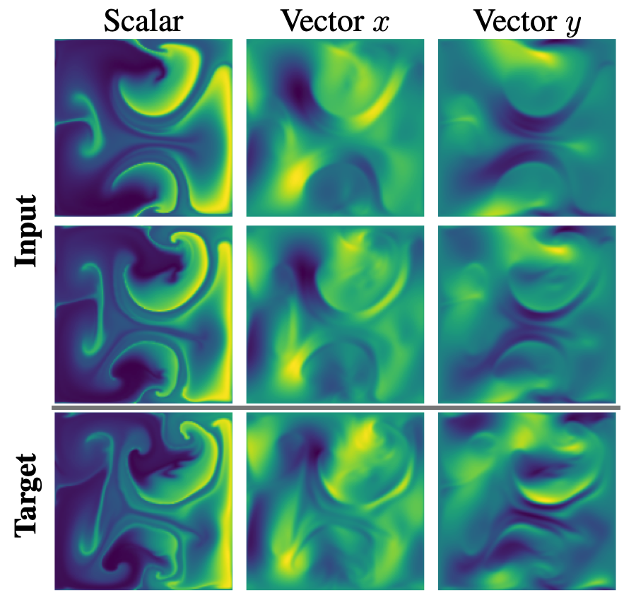
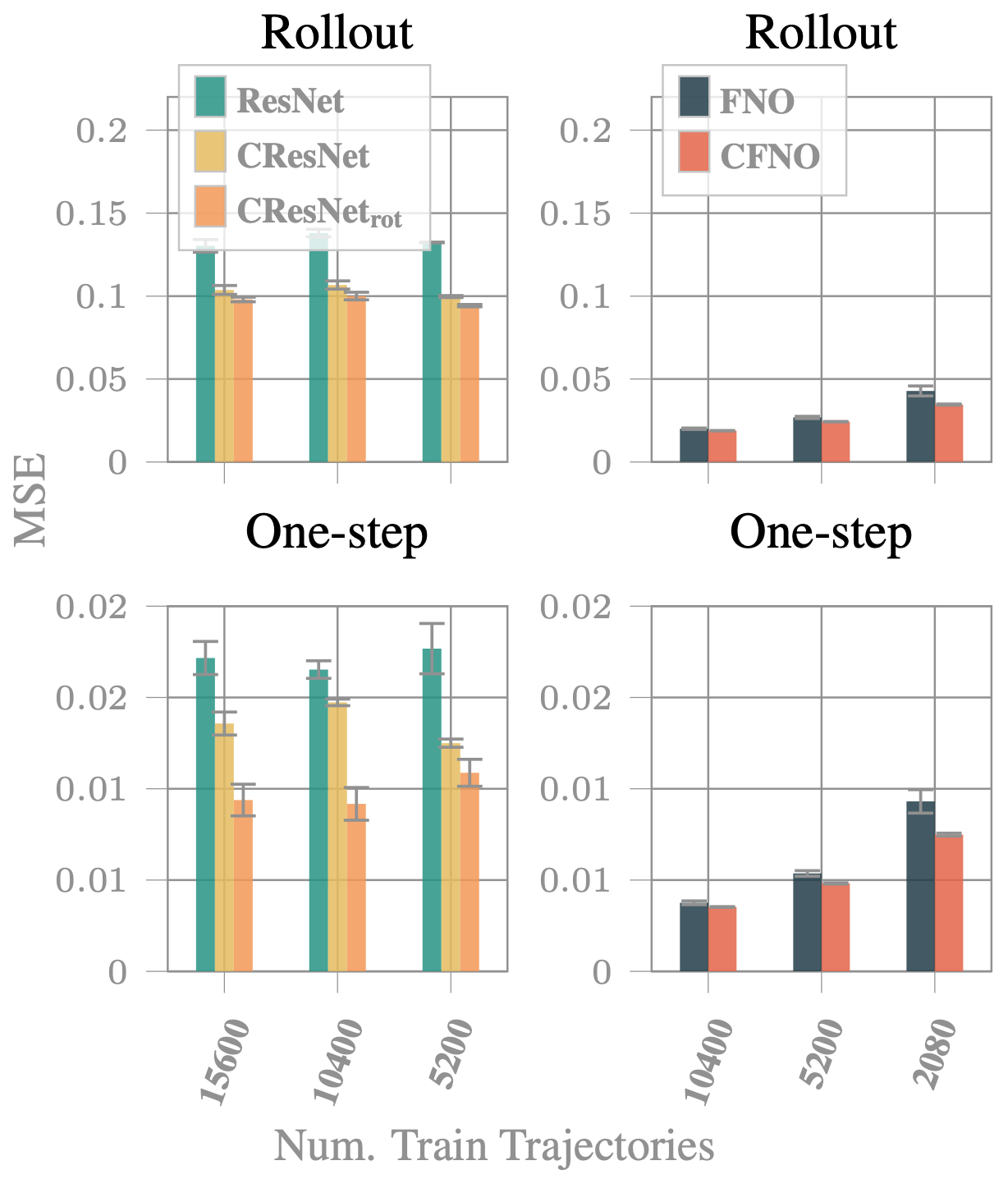
This particular system has a scalar field and a two-dimensional vector field. Since they are coupled by a PDE, it is natural and beneficial to encode them in the scalar and vector parts of a multivector, respectively. Hence, we work with the algebra $\Cl_{2, 0}(\mathbb{R})$. The bivector part of the algebra is left empty (zero) at the data input, but throughout the network the bivector part will get populated. The one-step loss denotes the error after a single iteration. The rollout loss shows the cumulative error when the network is autoreggresively applied. We see that the Clifford networks steadily outperform their naive counterparts. This makes them a promising candidate for such applications, potentially enabling fast and accurate PDE solutions to scientific problems in the near future.
Conclusion
In this post, we focused on the work Clifford Neural Layers for PDE Modeling (ICLR 2023). We introduced Clifford algebras and how to construct neural layers out of them. These generalize complex and quaternion neural networks and hence can tackle similar problems as they do, but even more. For example, they were shown to be of great value in approximating partial differential equation solutions by coupling the scalar and vector parts of the PDE in one multivector. The rotational layer is of particular interest, since it outperforms the native Clifford layer despite both being an equally flexible linear operation. In the next post of this series, we dive deeper into the geometry of this layer using modern (projective) geometric algebra. Let me know in the comments below if you have questions, comments, or ideas worth sharing!
Acknowledgments
I would like to thank Johannes Brandstetter, Jayesh Gupta, Marco Federici, and Jim Boelrijk for providing valuable feedback regarding this blogpost series.