C2C 4: Clifford Group Equivariant Neural Networks
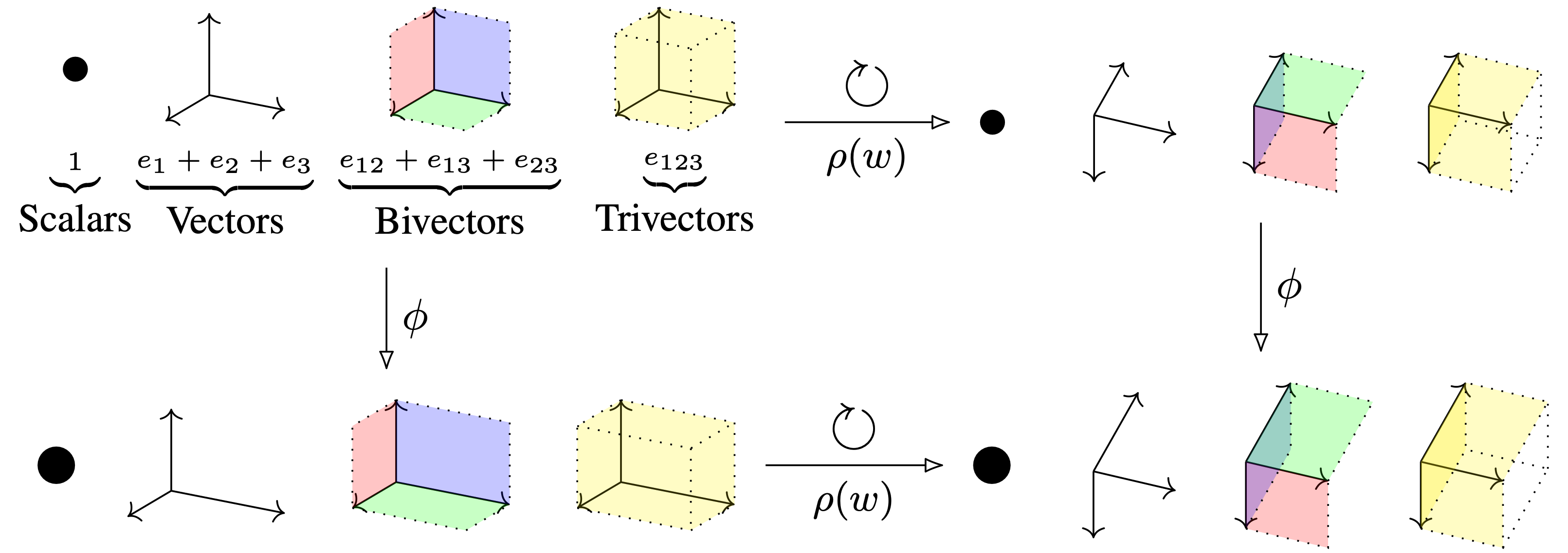
We have already arrived at the final post of this blog post series. In this version of multivector-valued networks, we ensure they obey an equivariance constraint. That is, the orientation of the problem should not matter for the prediction. Take for example the dynamics of the solar system. Our frame of reference (from which direction we observe the system) naturally does not affect its dynamics. For a neural network, this means that if we rotate a physical system, its representations should transform predictably. If the prediction is an invariant, say the total energy of the system, then it should remain unchanged. This is illustrated in the header figure. Here, $\phi$ represents the neural network and $\rho(w)$ an orthogonal transformation such as a rotation. We note that the order of operations does not matter. Thereby, the network is equivariant to rotations. Further, we see that the group action $\rho(w)$ respects the multivector grading. That is, the vectors, bivectors, trivectors are individually and consistently affected by the transformation.
A selection of papers that explores (modern) (hyper)complex neural networks architecture is Danihelka et al. (ICML 2016), Trabelsi et al. (ICLR 2018), Parcollet et al. (ICLR 2019), Tay et al. (ACL 2019), Zhang et al. (ICLR 2021), Brandstetter et al. (ICLR 2023), Ruhe et al. (ICML 2023), Ruhe et al. (2023), and Brehmer et al. (2023). These works are largely incremental; hence, we discuss them in this series in chronological order. The posts in this series are:
- C2C 1: Complex and Quaternion Neural Networks
- C2C 2: Clifford Neural Layers for PDE Modeling
- C2C 3: Geometric Clifford Algebra Networks
- C2C 4: Clifford Group Equivariant Neural Networks
If you are unfamiliar with the Clifford algebra, I highly suggest studying these in order. If anything is unclear, please let me know in the comments below, or get in touch with me directly!
In this post, we focus on the following work, which presents geometric algebra layers and their applications to dynamical systems tasks. Disclaimer: I am the first author.
Outline
- The Clifford Group. We identify a group and its action inside the Clifford algebra.
- Equivariant Operations. What operations are equivariant with respect to this group?
- Experiment: Lorentz Equivariance. An equivariant experiment in relativistic high energy physics.
- Conclusion. A wrapup and preview of what’s coming up next in this series.
The Clifford Group
This work is more technical than the previous works, and investigates the Clifford algebra from first principles. I suggest studying the previous posts first if you are unfamiliar with the Clifford algebra and typical constructions. Let $(V, q)$ be a quadratic space. Let $\Cl(V, q)$ denote its Clifford algebra.
We first define a specific map $\rho(w): \Cl(V, q) \to \Cl(V, q)$ that has
\[\rho(w)(x):= wx^{[0]}w^{-1} + \alpha(w)x^{[1]}w^{-1}\,,\]where $w \in \Cl^{\times}(V, q)$ is an invertible element. Let’s investigate this equation. First, we see a similar sandwich structure using geometric products as previously applied in the group action layers. However, it is split into two terms. The first part considers the even grades of $x$: $x^{[0]}$. That is, the scalars (grade 0), bivectors (grade 2), etc. The second part considers $x^{[1]}$: the odd grades (vectors, trivectors, etc). However, here, the action is twisted by the main involution $\alpha(w)$ which has $\alpha(w):= w^{[0]} - w^{[1]}$. I.e., it applies a minus sign to the odd grades. When $w$ is homogeneous, i.e., it only has nonzero odd or even grades, but not both at the same time, then one can also write
\[\rho(w)(x) := \begin{cases} w x w^{-1}, &w \in \Cl^{[0]}(V, q) \\ w\alpha(x)w^{-1}, &w \in \Cl^{[1]}(V, q),\end{cases}\]where $\Cl^{[0]}(V, q)$ denotes the even part of the algebra (the even grades) and $\Cl^{[1]}(V, q)$ the odd grades.
We can now construct a group, called the Clifford group, as follows:
\[\Gamma^{[\times]}(V, q) := \left \{ w \in \Cl^{[\times]}(V, q) \cap \left( \Cl^{[0]}(V, q) \cup \Cl^{[1]}(V, q) \right) \mid \forall v \in V, \rho(w)(v) \in V \right \}.\]Let’s dissect this. First, we consider only elements in $\Cl^{[\times]}(V, q)$, which denotes the invertible elements of the algebra. I.e., those $w$ such that there exists a $w^{-1}$ that has $w w^{-1} = 1$. Like matrices, not all elements of the algebra are invertible. Further, we require $w$ to be homogeneous, by taking the intersection with the fully even or odd elements of the algebra. Finally, we require $w$ to preserve vectors under the twisted conjugation. Relating things to the previous post, elements of the $\mathrm{Pin}$ group, generated by composing reflections, satisfy these requirements. For example, a vector $w \in V = \Cl^{(1)}(V, q)$ is a grade 1 element and therefore homogeneous. Applying the conjugation $-wvw^{-1}$, for $v \in V$, carries out a reflection as we saw before. I.e., the result is again a vector in $V$. Again, just like the previous post, we can just stack such conjugations, e.g., a rotation $w_2 w_1 v w_1^{-1} w_2^{-1}$, to obtain higher higher-order orthogonal transformations. It is clear to see that these preserve vectors. The definition of $\Gamma^{[\times]}(V, q)$ is slightly more general.
We designed $\rho(w)$ to have several favorable properties that we capture in the following big theorem.
- Additivity: $\rho(w)(x_1+x_2) = \rho(w)(x_1) + \rho(w)(x_2)$
- Scalar multiplicativity: $\rho(w)(c\cdot x) = c \cdot \rho(w)(x)$
- Multiplicativity: $\rho(w)(x_1x_2) = \rho(w)(x_1) \rho(w)(x_2)$
- Invertibility: $\rho(w^{-1})(x) = \rho(w)^{-1}(x)$
- Composition: $\rho(w_2) \left( \rho(w_1)(x) \right) = \rho(w_2w_1)(x)$
- Orthogonality: $b\left(\rho(w)(x_1),\rho(w)(x_2) \right) = b \left( x_1,x_2 \right) $
We use these properties to construct equivariant neural layers with respect to the Clifford group. However, by the last property (orthogonality) we see that the Clifford group acts as an orthogonal transformation! I.e., the Clifford group action preserves distances. Hence, by being equivariant with respect to the Clifford group, we are equivariant with respect to the orthogonal group (rotations, reflections, etc).
Equivariant Operations
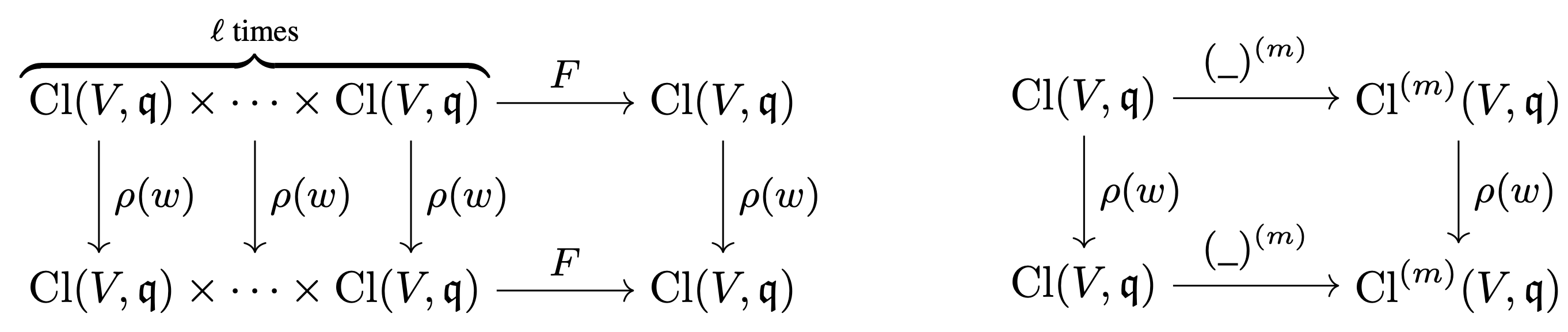
We prove Clifford equivariance of two rather fundamental operations: grade projections and polynomials. First, let’s discuss grade projections. We have
\[\rho(w)(x)^{(m)} = \rho(w)(x^{(m)}).\]Here, $\_^{(m)}$ denotes selecting the grade-$m$ part of a multivector (the scalar ($m=0$), vector($m=1$), bivector ($m=2$), etc). It is unaffected by the adjusted twisted conjugation. So, we can rotate first and then select the grade, or select first and then rotate. This is illustrated in the header figure: the vector, bivector, and trivector parts all transform independently. As such, it does not matter if we select one component first and then apply the transformation.
Next, we have equivariance with respect to polynomials. Let $x_1, \dots, x_\ell$ be a set of “steerable” multivectors. With steerable, we mean that these are all expressed in the same basis that transforms under $\rho(w)$. Let $F(x_1, \dots, x_\ell): \Cl(V, q)^\ell \to \Cl(V, q)$ be a multivariate polynomial in these multivectors. We have the property
\[\rho(w)(F(x_1, \dots, x_\ell)) = F(\rho(w)(x_1), \dots, \rho(w)(x_\ell)).\]That is, computing a polynomial in these multivectors is equivariant with respect to the Clifford group. Try to check this for yourself using a small example!
Clifford Equivariant Layers
The equivariance results allow us to parameterize a remarkable number of equivariant operations. In the following, let $x_1, \dots, x_\ell \in \Cl(V, q)$ be a set of steerable multivectors. As input data, they could be the positions of a set of planets. Using the standard three-dimensional basis we have
\[0 \cdot 1 + x_1 e_1 + x_2 e_2 + x_3 e_2 + 0 e_{12} + 0 e_{13} + 0 e_{23} + 0 e_{123},\]where $x_1, x_2, x_3$ are the spatial coordinates. That is, we leave the scalar, bivector, and trivector components to zero. These entries will get populated in the forward pass, though.
Linear Layers
First, we note that we can obtain linear layers by setting
\[y_{c_\text{out}}^{(k)} := T^{\text{lin}}_{\phi_{c_{\text{out}}}}(x_1, \dots, x_\ell)^{(k)} := \sum_{c_{\text{in}}=1}^\ell \phi_{c_{\text{out}}c_{\text{in}} k} \, x_{c_{\text{in}}}^{(k)},\]where $\phi_{c_{\text{out}}c_{\text{in}}k}$ is a scalar parameter. Note that we can apply a linear combination dependent on the grade $k$. This is because $\rho(w)$ respects the grading structure, as discussed above. Brehmer et al. then show that this comprises all Clifford equivariant transformations. It is easy to see that this map is equivariant, as a polynomial restricted to the first-order terms is exactly this transformation. By repeating this for multiple output channels, we obtain a fully-connected multivector-valued linear map.
Geometric Product Layers
The main merit of the current method is that we can also apply multiplicative operations such as the geometric product. We can parameterize a single geometric product as follows
\[P_\phi(x_1, x_2)^{(k)} := \sum_{i=0}^n \sum_{j=0}^n \phi_{ijk} \, \left( x_1^{(i)} x_2^{(j)}\right)^{(k)}.\]One can check the equivariance of this operation, as $\rho(w)$ respects linearity, products, scalar multiplication, and grade projections.
Since the algebra has $n+1$ grades, we have that every geometric product can therefore have $(n+1)^3$ parameters. In practice, however, many of these will invariably be zero due to the nature of the geometric product. For example, the geometric product of two vectors will not yield a new vector (but a scalar and a bivector). These will of course not be parameterized.
The squares and bivariate interactions of a polynomial $F(x_1, \dots, x_\ell)$ are such geometric products. There are, however, $\ell^2$ such terms. If $\ell$ is reasonably large, that will get rather expensive.
As such, we usually compute
\[y_{c_\text{out}}^{(k)} := T^{\text{lin}}_{\phi_{c_{\text{out}}}}(x_1, \dots, x_\ell), \quad c_{\text{out}} = 1, \dots, \ell \,,\]and apply pairwise geometric products \(z_{c_{\text{out}}} := P_\phi(x_{c_{\text{out}}}, y_{c_{\text{out}}})\).
Or, alternatively, we have fully-connected geometric product layers
\[z_{c_{\text{out}}}^{(k)}:= T^{\text{prod}}_{\phi_{c_\text{out}}} (x_1, \dots, x_\ell, y_1, \dots, y_\ell)^{(k)} := \sum_{c_{\text{in}}=1}^\ell P_{\phi_{c_{\text{out}} c_{\text{in}}}}(x_{c_{\text{in}}}, y_{c_{\text{in}}})^{(k)},\]which are more expensive but also more expressive.
Implementation
Here, we will discuss the implementation of these layers.
The official implementation can be found here
including a small tutorial.
We also have an interactive demo at
Google Colaboratory Tutorial: ![]()
Clifford Algebra Object
To work with the layers introduced above, we need to be able to represent and operate on multivectors. Let’s say we are in a two-dimensional space. We consider some vector data, e.g., the positions of a set of planets. Further, we have scalar features, e.g., the mass of the planets. We can represent this data as follows:
  algebra = CliffordAlgebra((1., 1.))
  h = torch.randn(1, 8, 1)  # 8 scalar features
  x = torch.randn(1, 8, 2)  # 8 vector features, note that we have 2 dimensions.
We have a batch dimension of 1. We create a Clifford algebra object by passing the signature of the quadratic form. Since it has two positive entries, we are in a two-dimensional Euclidean space.
To embed the data into the algebra, we use the embed_grade method.
h_cl = algebra.embed_grade(h, 0)
x_cl = algebra.embed_grade(x, 1)

input = torch.cat([h_cl, x_cl], dim=1)
We embed the scalar features into the scalar part of the algebra and the vector features into the vector part, which are the 0 and 1 grades, respectively. Then we concatenate the two parts to obtain the input data.
At the end of our neural network (layer on) we want to extract scalar or vector data to make our predictions. For those, we can use algebra.get_grade.
We can now operate on this data using $\rho(w)$: the Clifford group action.
The goal is that the network respects (i.e., is equivariant or invariant with resepct to) this action.
Remember, $\rho(w)$ represents a rotation, reflection, or other orthogonal transformation.
To create orthogonal representations, we use the versor method, which composes reflections, leading to orthogonal transformations.
# Reflector
v = algebra.versor(1)

# Rotor
R = algebra.versor(2)
A 1-versor is a reflection, where two reflections (2-versor) compose to a rotation.
We can create reflected and rotated versions of the input data as follows:
input_v = algebra.rho(v, input.clone())

input_R = algebra.rho(R, input.clone())
Other common multivector operations are also available; see the official repository for more details.
Linear Layers
We inspect the forward method of the linear layer implementation.
    def _forward(self, input):
        return torch.einsum("bmi", input, self.weight)

    def _forward_subspaces(self, input):
        weight = self.weight.repeat_interleave(self.algebra.subspaces, dim=-1)
        return torch.einsum('bmi, nmi->bni', input, weight)

    def forward(self, input):
        result = self._forward(input)

        if self.bias is not None:
            bias = self.algebra.embed(self.bias, self.b_dims)
            result += unsqueeze_like(bias, result, dim=2)
        return result
self._forward is set dependent on whether we want a linear combination in each grade (subspace) or on the entire multivectors.
Usually, one wants the former, and efficiency gains by operating on entire multivectors together are insignificant.
We use torch.einsum to efficiently implement the operation.
Inspecting the einsum signature, we see that we go from m channels to n channels, for each Clifford grade i.
Finally, we can add a bias term to the zero subspace. To achieve $\mathrm{SO}(n)$-equivariance (as opposed to $\mathrm{O}(n)$), one can also add a learned pseudoscalar bias term.
Geometric Product Layers
We inspect the forward method of the element-wise geometric product layer implementation.
        input_right = self.linear_right(input)
        input_right = self.normalization(input_right)

        weight = self._get_weight()

        if self.include_first_order:
            return (
                self.linear_left(input)
                + torch.einsum("bni, nijk, bnk -> bnj", input, weight, input_right)
            ) / math.sqrt(2)

        else:
            return torch.einsum("bni, nijk, bnk -> bnj", input, weight, input_right)
Given our inputs, we first linearly transform them to get a new set of multivectors.
One can imagine a permutation of the input channels.
Then, we normalize the right-hand side of the geometric product to avoid numerical instabilities throughout the network.
This, as described in the paper, is a learned normalization.
Alternatives, such as regular multivector normalization or no normalization at all sometimes also work, and more exploration would be useful here.
Finally, we compute the geometric products using torch.einsum.
As such, we get multiplicative interaction between the input channels.
If self.include_first_order is set to True, we also apply another linear to get a full polynomial up to the second order.
Note that we compute element-wise geometric products here. We also have a fully-connected version of this, where we compute the geometric product between all pairs of input channels.
Multivector Sigmoid Linear Units
The final layer we discuss here is the multivector sigmoid linear unit (MVSiLU). Its forward map is given by
    def forward(self, input):
        norms = self._get_invariants(input)
        norms = torch.cat([input[..., :1], *norms], dim=-1)
        a = unsqueeze_like(self.a, norms, dim=2)
        b = unsqueeze_like(self.b, norms, dim=2)
        norms = a * norms + b
        norms = norms.repeat_interleave(self.algebra.subspaces, dim=-1)
        return torch.sigmoid(norms) * input
Here, we first get the invariants of the input multivectors.
The first subspace is always invariant, so we don’t compute its magnitude but just concatenate it to the rest.
We can then apply any scalar function to the invariants.
Here, we just scale and shift them and apply a sigmoid, but for more expressive power, one could also use a neural network MLP!
We apply this technique in some experiments.
Equivariant Neural Networks
By combining layers as presented above, we can create equivariant Clifford neural networks.
We can even create more exotic architectures, such as GNNs, Transformers, and so on.
So long as all operations are equivariant, the network will be equivariant.
For GNNs, for example, the message passing reduction is usually a sum or mean, which both are equivariant.
We also have an interactive demo at
Google Colaboratory Tutorial: ![]()
Experiment: Lorentz-equivariant Top Tagging
One very nice property of Clifford equivariant networks is that we can be invariant or equivariant with respect to the orthogonal transformations of any quadratic space. That includes the Minkowski space of Einstein’s special relativity. The orthogonal transformations of this space are captured by the Lorentz group $\mathrm{O}(1, 3)$. That is, the metric $M$ is given by $M:=\mathrm{diag}(1, -1, -1, -1)$. This changes the way distances (norms, inner products) are calculated in the space. Namely, for two vectors $u, v \in \mathbb{R}^4$, we have $\langle u, v \rangle = u^T M v$, where the metric acts in the middle. In the Euclidean space, the metric is the identity matrix, and the inner product is the standard dot product.
This group captures the effect that moving at a fixed velocity changes one’s perception of a phenomenon. That is, the laws of physics should be invariant to the inertial frame of reference. These perceptual distortions such as relativity of simultaneity, length contraction, and time dilation, are only significant when moving at relativistic speeds.
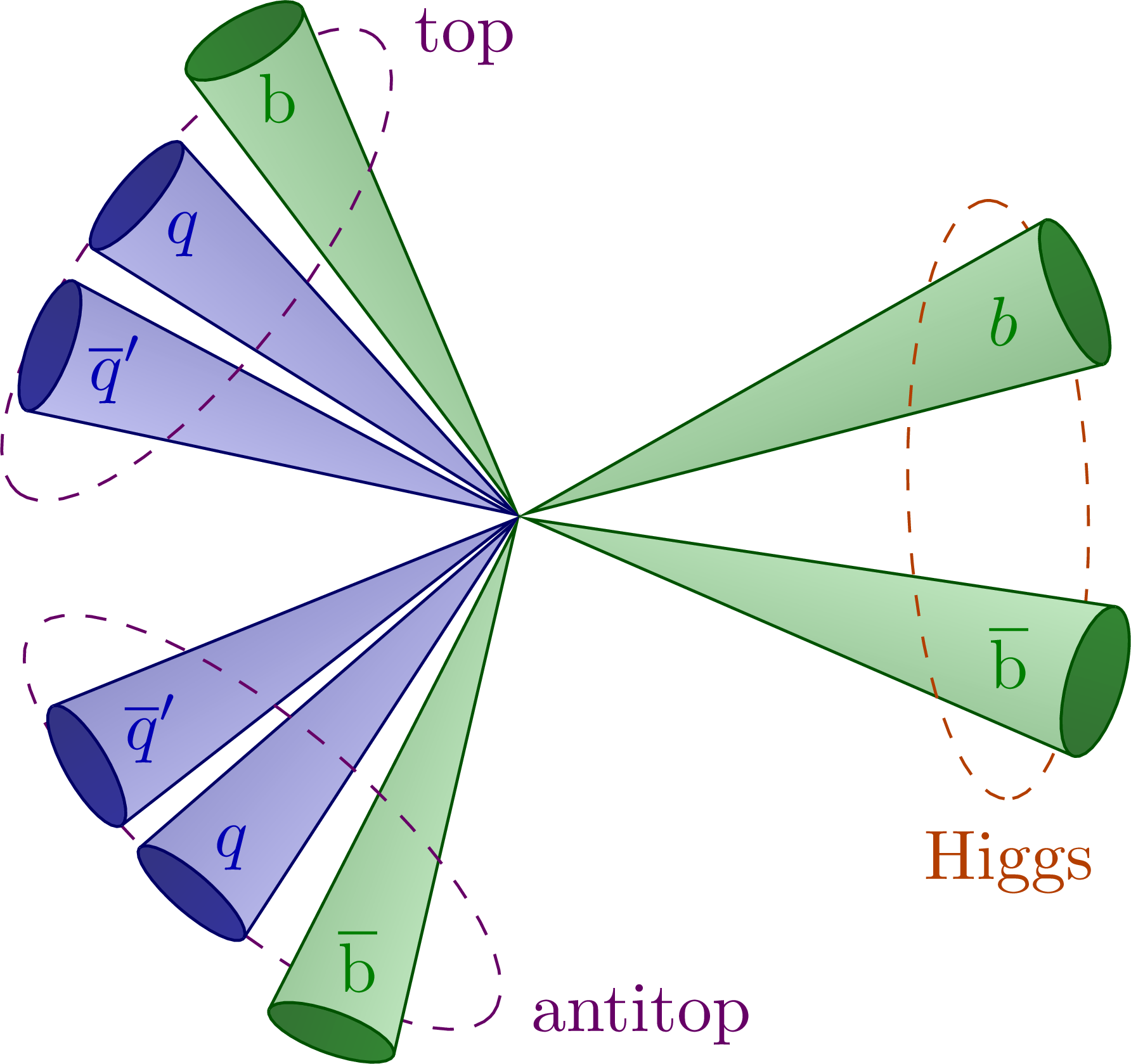
Such extreme environments are relevant for the experiments carried out at, e.g., CERN’s Large Hadron Collider (LHC). One such experiment is jet tagging. Jet tagging in collider physics is a technique used to identify and categorize high-energy jets produced in particle collisions. By combining information from various parts of the detector, it is possible to trace back the origin of these jets and classify them. The current experiment seeks to tag jets arising from the heaviest particles of the standard model: the “top quarks”. A jet tag should be invariant with respect to the reference frame in which the jet is observed, whereas the frames themselves change under Lorentz boosts due to the relativistic nature of the particles.
In the table below we consider a benchmark often used for tagging such jets.
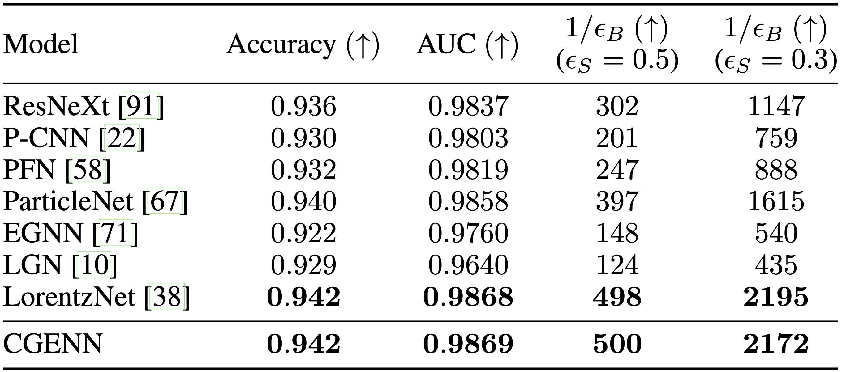
We note that we outperform many baselines and perform equally well as a state-of-the-art method. This is quite remarkable, since most of these were specifically designed for the task, whereas our method is rather general. That is, we also perform equivariance experiments for three- and five-dimensional orthogonal groups.
Conclusion
In this final post, we investigated a group inside the Clifford algebra that always acts orthogonally: the Clifford group. By analyzing its action, we identified several favorable properties. These allow us to build equivariant neural layers from two fundamental operations: polynomials and grade projections. Clifford equivariant neural layers then allow us to parameterize nonlinear maps that respect orthogonal transformations in any quadratic space. Despite this generality, we were able to get highly promising experimental results. These are (to us) very exciting developments that open up a new line of research.
We have arrived at the end of the blog post series! Starting at complex neural networks, we made generalizations to quaternion and then Clifford hypercomplex neural networks. Then we incorporated a more geometric inductive bias by inspecting and generalizing the rotational layer. This was done in the geometric algebra post. Finally, we realized how to enforce equivariance and invariance constraints that modern physics builds on. This allows for robust and predictable results that respect the invariances that we observe in the real world. The development from complex neural network to Clifford equivariant neural layers is very interesting but - although in hindsight rather logical - I would never have guessed where we ended up. And also in such a high pace! I’m very curious in what the (near) future might bring. Let me know in the comments below if you have ideas or questions worth sharing!
Acknowledgments
I would like to thank Johannes Brandstetter, Jayesh Gupta, Marco Federici, and Jim Boelrijk for providing valuable feedback regarding this blogpost series.