C2C 3: Geometric Clifford Algebra Networks
We concluded the previous article with a slightly specialized version of Clifford neural layers: the rotational layer. Though equally flexible, this layer empirically yielded better performing models for neural PDE surrogates. A potential reason for this might be that the rotational layer applies more valid geometric transformations in comparison to geometric product layers. The geometric product of two multivectors is hard to interpret because it mixes grades (scalars, vectors, bivectors, etc.) in an abitrary way. Thereby, the intended geometric bias may not be as strong as one might hope. In this paper, motivated by the rotational layer, we explore the geometric side of the Clifford algebra deeper, diving into modern plane-based geometric algebra. We will construct geometrically inspired linear layers (group action layers) as well as nonlinearities and apply them to point-cloud based tasks and neural PDE surrogates. We show, through better performing empirical results, that strengthening this geometric bias is indeed advantageous.
A selection of papers that explores (modern) (hyper)complex neural networks architecture is Danihelka et al. (ICML 2016), Trabelsi et al. (ICLR 2018), Parcollet et al. (ICLR 2019), Tay et al. (ACL 2019), Zhang et al. (ICLR 2021), Brandstetter et al. (ICLR 2023), Ruhe et al. (ICML 2023), Ruhe et al. (2023), and Brehmer et al. (2023). These works are largely incremental; hence, we discuss them in this series in chronological order. The posts in this series are:
- C2C 1: Complex and Quaternion Neural Networks
- C2C 2: Clifford Neural Layers for PDE Modeling
- C2C 3: Geometric Clifford Algebra Networks
- C2C 4: Clifford Group Equivariant Neural Networks
If you are unfamiliar with the Clifford algebra, I highly suggest studying these in order. If anything is unclear, please let me know in the comments below, or get in touch with me directly!
In this post, we focus on the following work, which presents geometric algebra layers and their applications to dynamical systems tasks. Disclaimer: I am the first author.
Outline
- Plane-based Geometric Algebra. An introduction to geometric algebra and its isometries.
- Geometric Algebra Networks. How to construct geometric Clifford neural layers?
- Experiment: Tetris. An analysis of a rigid body dynamics experimet.
- Experiment: Shallow-Water Equations. Modeling the shallow-water equations using geometric Clifford networks.
- Conclusion. A wrapup and preview of what’s coming up next in this series.
Plane-based Geometric Algebra
We have introduced last time a simple construction of the Clifford algebra, without paying much attention to how it can be used in a more geometric fashion. Clifford algebra is not synonymous with geometric algebra for no reason 😉. Specifically, we investigate the isometries (metric-preserving transformations) of the algebra. To this end, we introduce the Pin group and its Clifford representations. But to get there, we first have to discuss a rather fundamental operation: the reflection.
Reflections
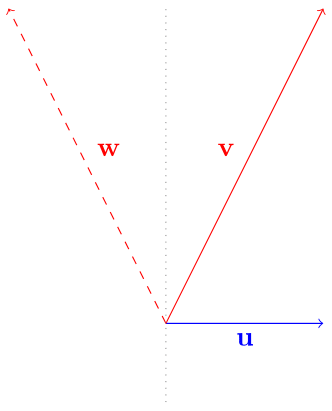
We consider the three-dimensional geometric algebra $\Gbb_{3}$ or, using the notation of the previous post, $\Cl_{3, 0}(\Rbb)$. A vector $u$ expressed in a basis ${e_1, e_2, e_3}$ in this algebra gets can be written as
\[\mathbf {u} := u_1 e_1 + u_2 e_2 + u_3 e_3 \,.\]Let $\bf u, \bf v \in \Gbb_{3}$ be such vectors. It can be shown that a reflection, as understood from linear algebra, can be rewritten using the geometric product into
\[\bf w := u[v] := - u v u^{-1} \,. \tag{1}\]I.e., this operation reflects the vector $\mathbf v$ in the hyperplane normal to $\mathbf u$.
There are many noteworthy similarities of this operation to group conjugation, which can be understood as a group acting on itself. Specifically, for the abstract reflection group $R$, one could take two reflections $u, v \in R$ and obtain
\[w:= uvu^{-1} \,,\]where $w \in R$ is a “reflected version of v”. That is, it is the reflection obtained after reflecting $v$ in $u$. An analogy of this: the act of writing one’s name upside-down can be decomposed into inverting the page, then writing, and then invert back.
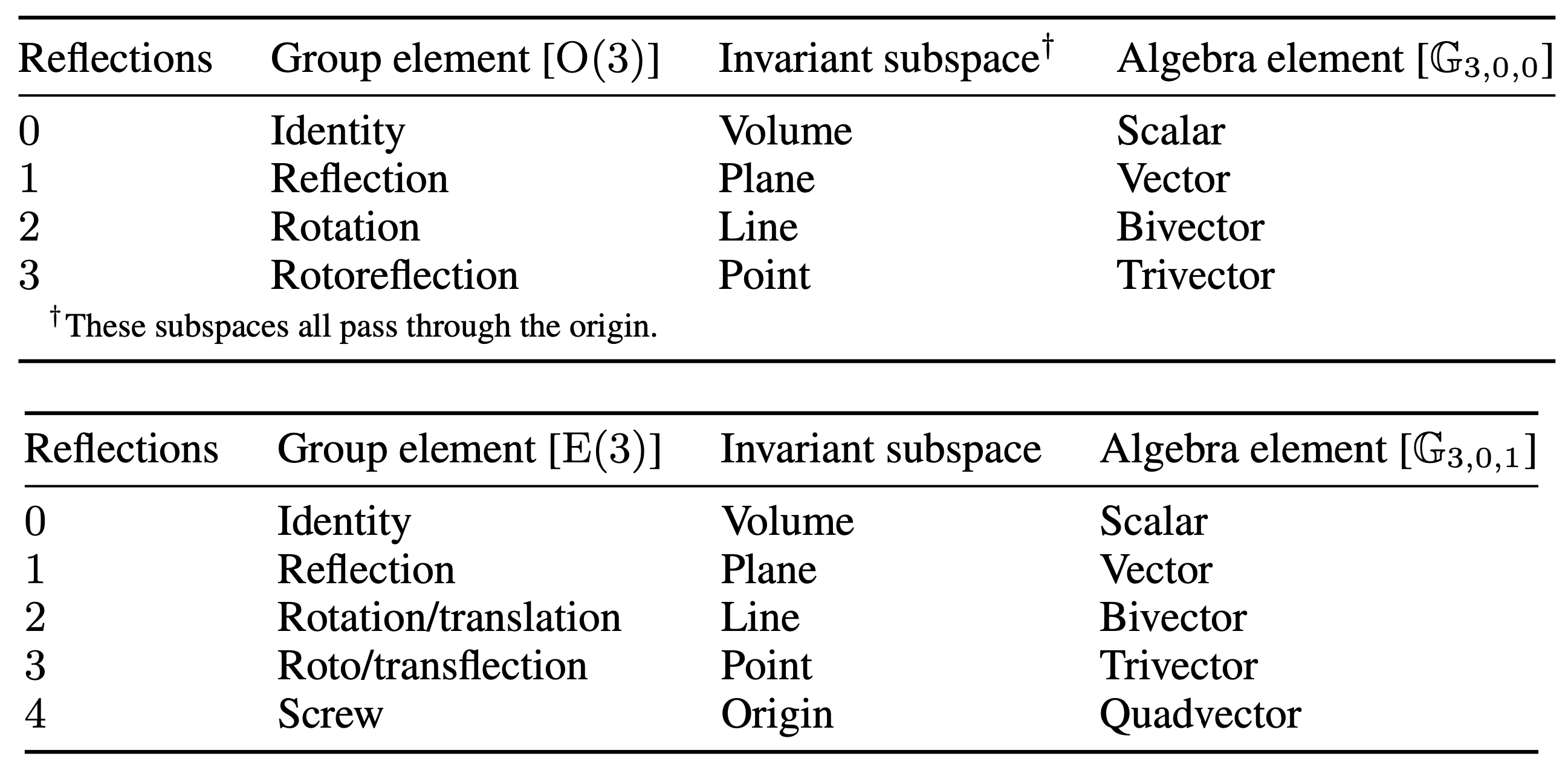
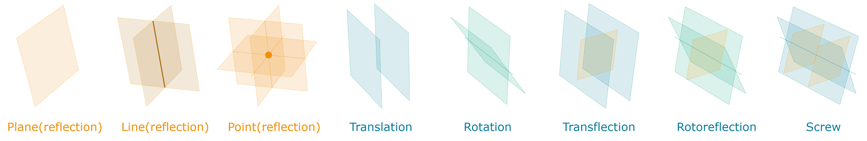
Now, in the geometric algebra version, we saw that we can use vectors and the geometric product to apply a reflection. The resulting $\bf w$ is also a vector. Hence, this element can be used to carry out a new reflection. It should become clear that vectors are representations of elements in the reflection group! Now, as also discussed, Equation 1 exactly reflects $\bf v$ in the hyperplane normal to $\bf u$. I.e., $\bf u$, a vector, also defines a hyperplane. We thus get that vectors represent reflections and hyperplanes. I.e., they are algebraic elements, “arrows” (as used in physics), transformations (reflections), and Euclidean elements (planes), all at the same time! We will build upon this insight in the following sections.
The Pin group.
The famous Cartan-Dieudonné theorem states that any orthogonal transformation of any quadratic space can be decomposed into a series of reflections. For example, two reflections lead to a rotation (see figure below).
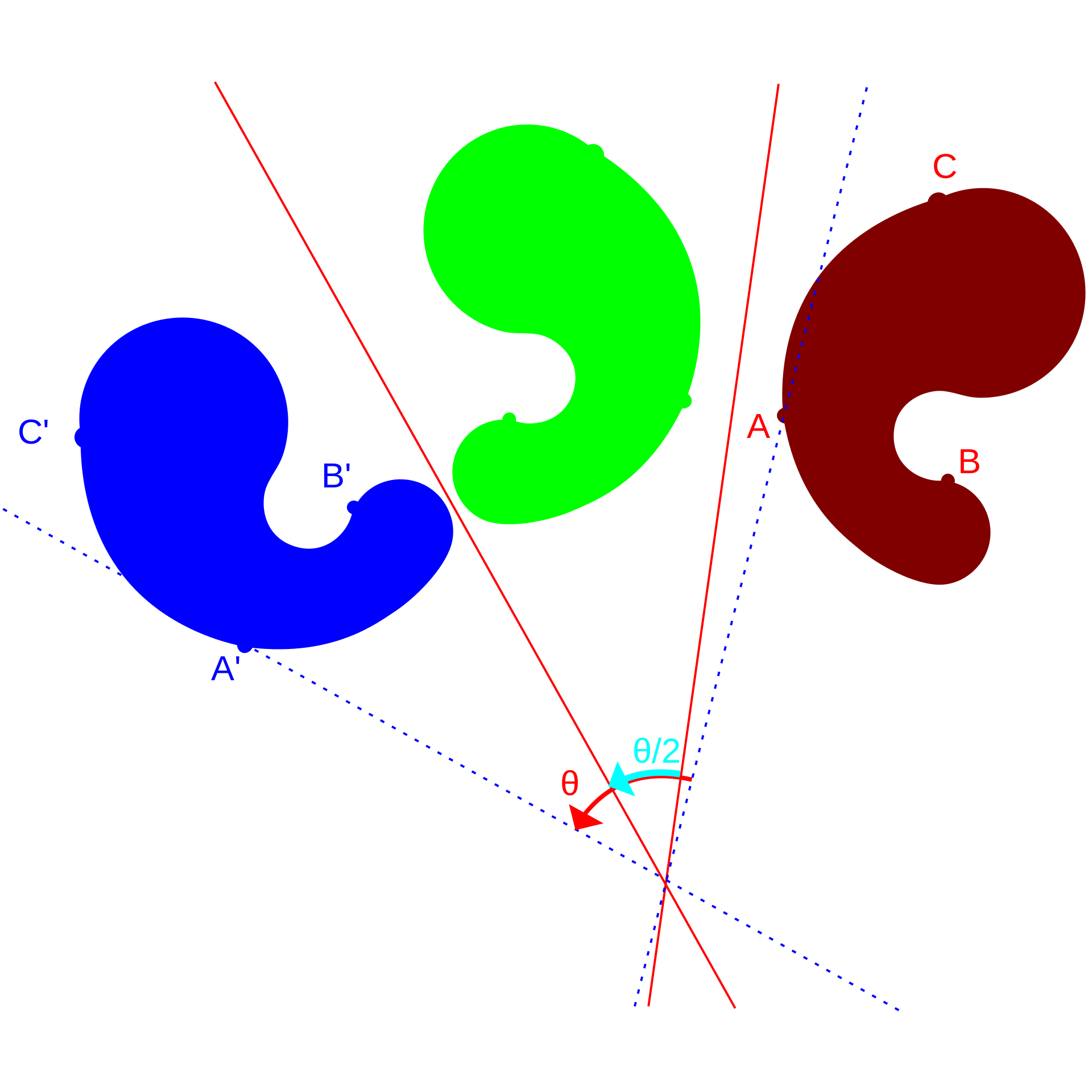
The group of composed reflections is called the Pin group, and it is usually directly defined using its representation in the Clifford algebra. I.e., every $u \in \mathrm{Pin}$ has $u=u_1 \dots u_k$, where $u_i$ is a reflection. Using the representation of a reflection in the geometric algebra as a vector, we thus get for a rotation
\[\mathbf v \mapsto \mathbf u_2 \mathbf u_1 \mathbf v \mathbf u_1^{-1} \mathbf u_2^{-1} = (\mathbf u_1 \mathbf u_2) \mathbf v (\mathbf u_1 \mathbf u_2)^{-1} \,, \tag{2}\]where we applied the sandwich structure twice. The associativity of the geometric product allows us to group (pre-compute) the vector composition first. Recall from the previous post that the geometric product of two vectors yields scalar and bivector parts. Since Equation (2) composes two reflections leading to a rotation, bivectors thus parameterize rotations. Note that $\mathbf u_1 \mathbf u_2$ is a representation of a $\mathrm{Pin}$ element.
Applying $k$ reflections ($\mathbf u := \mathbf u_1 \dots \mathbf u_k$) yields
\[(-1)^k \mathbf u \mathbf v \mathbf u^{-1}\,,\]which, by the theorem, is a valid orthogonal transformation. In fact, the Pin group is the double cover of the orthogonal group (for a nondegenerate vector space over the real numbers). To see this, note that $\mathbf u$ and $-\mathbf u$ lead to the same transformation.
Let’s summarize our findings so far. We set out on an investigation of the geometry of a Clifford algebra. By the Erlangen program, geometry is fundamentally related to the isometries of a space. Using the Cartan-Dieudonné theorem, one can obtain all such transformations by their fundament: the reflection. We investigated a natural representation of reflections in the algebra, noting that vectors parameterize reflections, hyperplanes, and arrows at the same time. It was rather straightforward to compose reflections, leading to rotations and higher-order orthogonal transformations. These all have a representation in the algebra. For rotations, they turned out to consist of bivectors. Let’s now go a step further and study a rather recent innovation in the world of geometric algebra: the projective geometric algebra.
Projective Geometric Algebra
The projective geometric algebra (see also Roelfs & de Keninck, who also pioneered some of these ideas) was recently developed to carry out (computational) Euclidean geometry using similar notions as above. In order to do so, we need to free ourselves from a fixed origin. Specifically, note that every vector in the usual three-dimensional algebra $\Gbb_3$ is, like in linear algebra, fixed at the origin. Recall that a vector defines a plane through the origin or, equivalently, every plane has a normal vector:
\[ax + by + cz = 0 \leftrightarrow \mathbf n := [a, b, c]^\top \,,\]where the left equation describes a plane through the origin of three-dimensional space. We can offset this plane from the origin by adding some bias value \(\delta\)
\[ax + by + cz + \delta = 0 \leftrightarrow \mathbf n := [a, b, c, d]^\top \,,\]The induced normal vector, however, should carry the same magnitude as the original. All we did, after all, is just shift it.
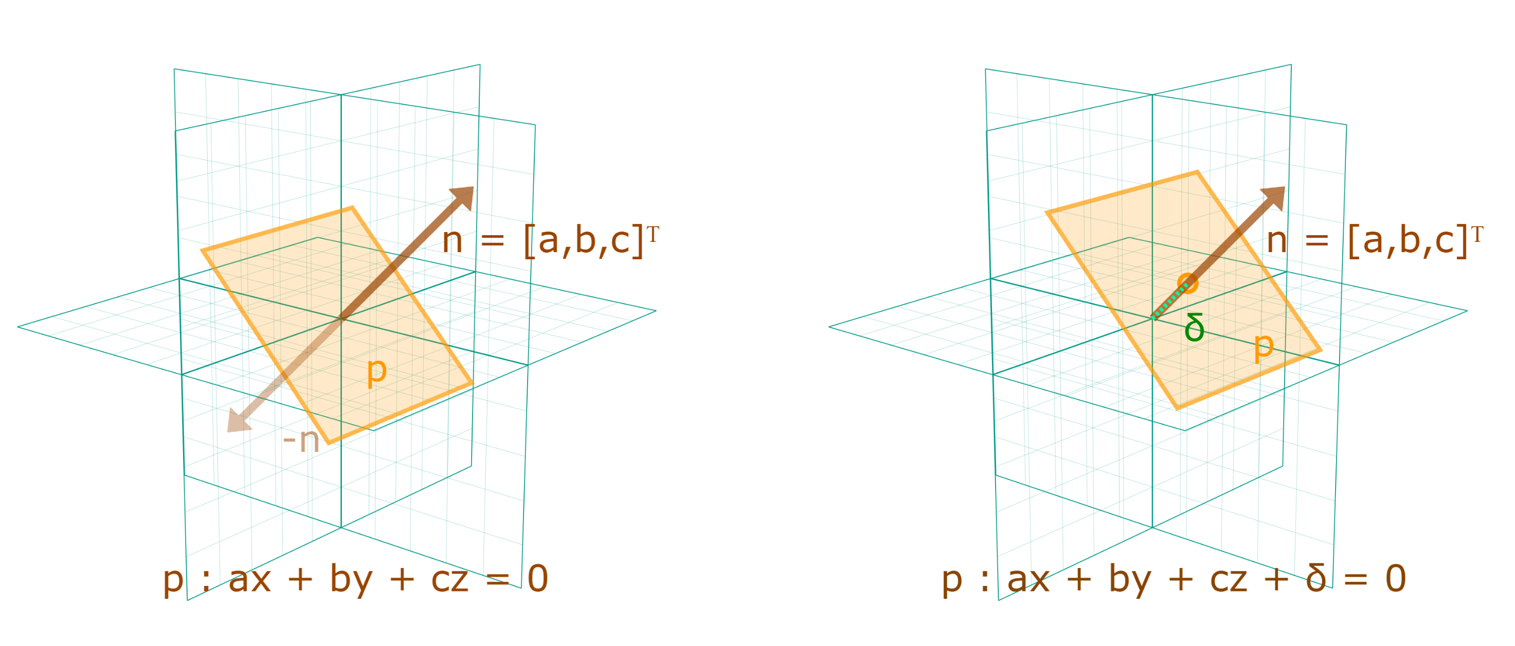
This motivates this fourth dimension to be a null vector. I.e., we pick a basis such that
\[\mathbf n := ae_1 + be_2 + ce_3 + \delta e_0 \,,\]where $e_0^2=0$. This ensures that \(\mathbf n\)’s magnitude is unchanged! The algebra is now denoted $\Gbb_{3, 0, 1}$ or, in the previous notation $\Cl_{3, 0, 1}(\Rbb)$.
Recall that isometries could be decomposed into compositions of reflections by the Cartan-Dieudonné theorem. Further, these reflections were parameterized with vectors defining hyperplanes through the origin. In the projective geometric algebra, we can move planes away from the origin. This allows us to create parallel planes. These parameterize translations!

By including this fourth null vector, even translations are captured by the composition of reflections and therefore by the sandwich product discussed before. I.e., we have incorporated the whole Euclidean group $E(3)$ in the framework.
Representing data structures
We already touched upon the notion that vectors can represent both transformations (reflections) as well as elements (Euclidean planes). This idea can be generalized. Specifically, the Euclidean elements are exactly the invariant subspaces of the transformations. For example, a reflection leaves a plane invariant. Similarly, rotations leave lines invariant. We saw that rotations are parameterized by bivectors. That means that bivectors parameterize lines. Rotoreflections (trivectors, i.e., products of three vectors) leave only points invariant. Points are therefore represented with trivectors.
Geometric Algebra Networks
We have investigated the geometry of the Clifford algebra much closer. Let’s take a step back and look into neural network parameterizations. In the Clifford layers post, we saw how the rotational layer looked really promising. In geometric algebra notation, we generalize this to a group action layer
\[\mathbf x \mapsto T_{g, w}(\mathbf x) := \sum_{i=1}^c w_i \cdot \mathbf a_i \mathbf x_i \mathbf a_i^{-1} \,,.\]Let’s digest what’s going on. The input $\mathbf x:=(\mathbf x_1, \dots, \mathbf x_c), \mathbf x_i \in \Gbb_{p, q, r}$ is a series of multivectors. E.g., a set of lines, planes, or points. Similarly to all the previous hypercomplex networks, we take linear combinations of some sort of product. In this case, that is the sandwich product, carrying out a Pin group action. In this work we focus on Spin actions (i.e., those $k$-reflections where $k$ is divisible by 2). These preserve the handedness of the space - for example, we exclude reflections. Then, we have learnable scalar weights $w_i \in \mathbb{R}$ that combine the actions. Further, the specific group actions $\mathbf a_i$ are also learned by learning the coefficients that carry out the action. For example, the bivector and scalar components, as we saw, compute rotations. So freely learning those yield rotational layers.
These layers are highly similar to the rotational Clifford layer, but induce an even stronger bias. We respect the nature of the data $\mathbf x_i$ and ensure it transforms in a geometrically valid way. That is, vectors will always remain vectors. Planes, lines and points always remain as such. We do not have arbitrary mixing between grades. Hence, we call networks constructed from these layers geometric templates that guide the transformation of, e.g., a dynamical system from timestep $t$ to $t+1$.
Implementation
    def forward(self, input):
        M = self.algebra.cayley
        k = self.action
        k_ = self.inverse(k)
        x = self.algebra.embed(input, self.input_blades)
        x[..., 14:15] = self._embed_e0
        # x[..., 14:15] = 1

        k_l = get_clifford_left_kernel(M, k, flatten=False)
        k_r = get_clifford_right_kernel(M, k_, flatten=False)

        x = torch.einsum("oi,poqi,qori,bir->bop", self.weight, k_r, k_l, x)

        x = self.algebra.get(x, self.input_blades)

        return x
def get_clifford_left_kernel(M, w, flatten=True):
    o, i, c = w.size()
    k = torch.einsum(f"ijk, pqi->jpkq", M, w)
    if flatten:
        k = k.reshape(o * c, i * c)
    return k


def get_clifford_right_kernel(M, w, flatten=True):
    o, i, c = w.size()
    k = torch.einsum(f"ijk, pqk->jpiq", M, w)
    if flatten:
        k = k.reshape(o * c, i * c)
    return k
This layer has been released at https://github.com/microsoft/cliffordlayers/blob/main/cliffordlayers/nn/modules/gcan.py
In the top panel, we see the forward function of a MultiVectorLinear class.
First, the algebra’s cayley table is invoked.
This is a sparse tensor that can be used to compute geometric products, and it is generated by a CliffordAlgebra class.
We then assign the group actions ($\mathbf a_i$ in the math above) to a variable $k$.
Next, we embed the data in the algebra, given a set of input blades.
E.g., to achieve Euclidean motions (including translations) we embed the data in the trivector components.
Next, we embed the $\delta$ coefficient of the $e_0$ plane (the offset from the origin, see above).
Then, to compute the left multiplication kernel for $\mathbf a_i$ and the right kernel for its inverse $\mathbf a_i^{-1}$.
The group action is then carried out by a big Einstein summation.
Finally, we get the resulting blades, which are by design always the same as the input blades.
Again, this is different from the geometric product layers of the previous post; they arbitrarily mixed blades.
In the second panel we see the left and right kernel functions. These carry out the same operation as in the previous post but in a more general/automatic way. I.e., in the previous posts about quaternion and Clifford neural networks we hand-constructed the kernels by concatenation and applying the correct minus signs. Here, the algebra’s Cayley table does that for us.
Nonlinearities
Next, we need some nonlinearities to enable the model to represent a richer function class. However, we must be careful not to lose the geometric inductive bias that was so carefully achieved through the group action layers. We took inspiration from the equivariance literature by applying nonlinear scaling to the hidden states. That is, we can put
\[[\mathbf x]_k \mapsto \sigma(f([\mathbf x]_k)) [\mathbf x]_k,\]where $[\cdot ]_k$ denotes the grade-$k$ part of the multivector. Here, since our models are not equivariant, $f$ can be an arbitrary function from \(\Gbb_{p, q, r}\) to \(\Rbb\). We then apply a sigmoid unit for stability reasons. The resulting function resembles a gated sigmoid linear unit (SiLU) or swish activation, but now multivector-valued.
Experiment: Tetris
Geometric Clifford Algebra Networks (GCANs) were specifically designed for modeling dynamical systems of (Euclidian) spaces. In order to test our parameterizations, we set up a synthetic experiment where certain rigid objects undergo several transformations. Specifically, we place Tetris figures at the origin, and sample random directions, velocities, rotation axes, and angular velocities. We apply these transformations to obtain a scene.
The goal is to predict, given a few input time-steps, the motions in the rest of the scene.
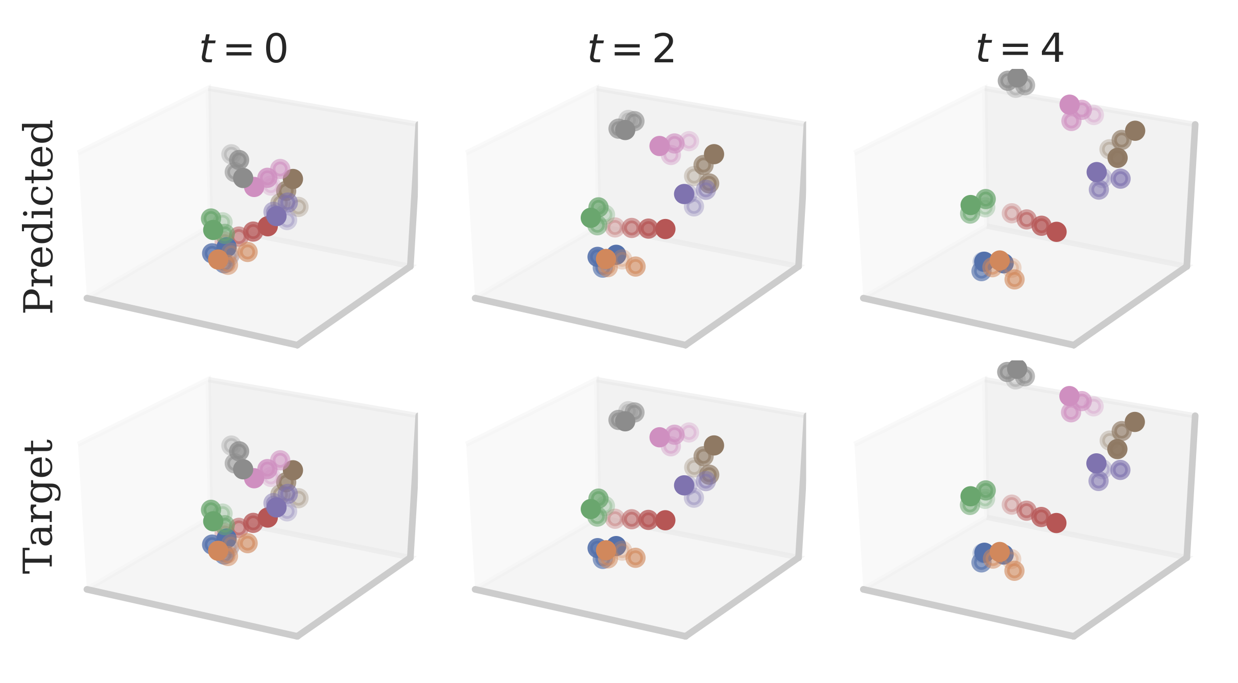
These are Euclidean motions and hence we use the projective geometric algebra $\Gbb_{3, 0, 1}$, which includes translations as parallel reflections. From the figure one qualitatively sees that the network is able to predict the dynamics quite well.
Experiment: Shallow-Water Equations
In this second experiment we continue the experiments from the Clifford neural layers paper, but with this new more geometrically inspired parameterization. Here, the vector field does not translate and we can therefore stick to $\Gbb_3$. The sandwich product in this algebra effectively carries out a rotation. Hence, we can make use of the rotational layer as introduced in the last post. However, this time we do not augment it with a geometric product for the scalar part and we use activations and normalizations that preserve the vector structure, as discussed above.
Using these convolutional layers, we introduce UNet-type architectures, as they prove to be highly accurate at modeling PDEs.
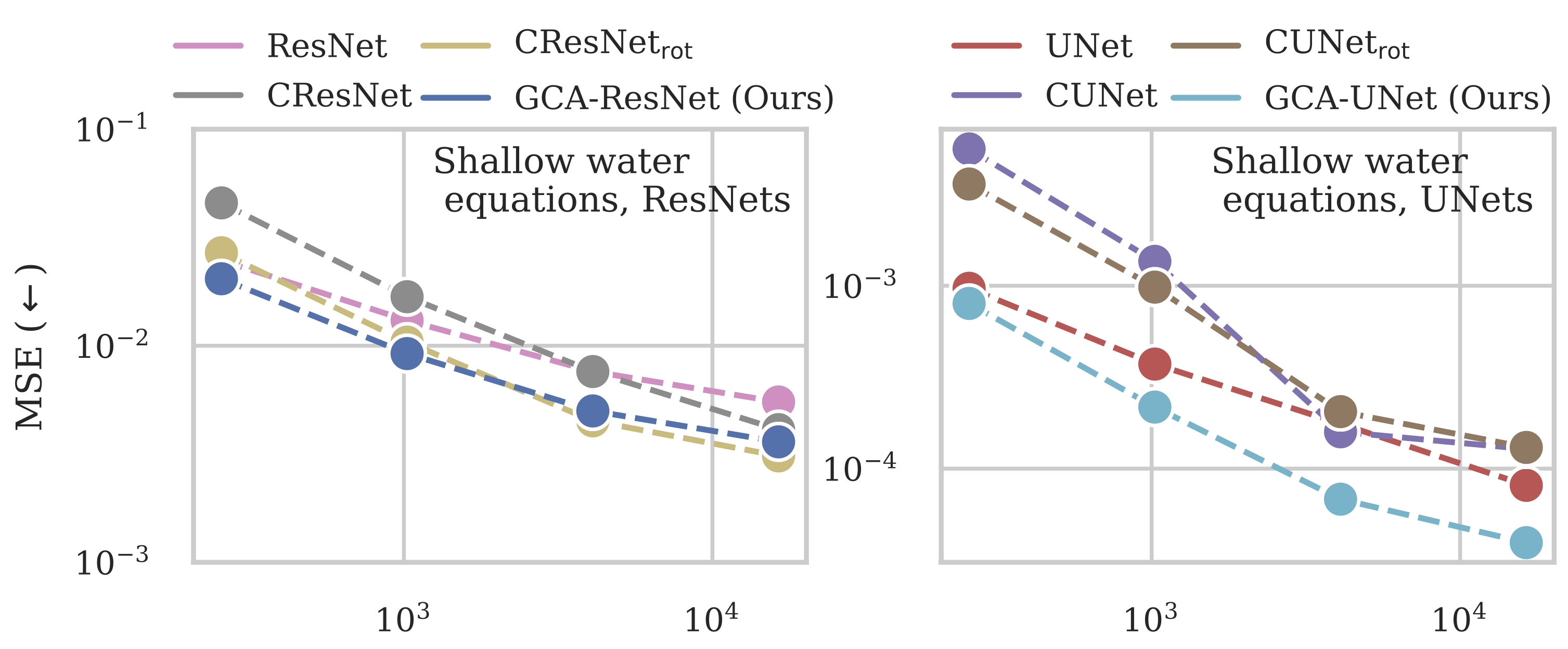
From the figure we see that, especially for the UNet architectures, the geometric inductive bias proves to be effective. We like to stress that these networks are rather big, having more than 50 million parameters, making them one of the few cases where geometry is incorporated at such scale.
Conclusion
Motivated by the success of the Clifford rotational layer for PDE solving, we explored the geometric side to the Clifford algebra more closely. In doing so, we realized that all isometries of any quadratic space can be achieved by composing reflections. In the projective geometric algebra, these isometries even include translations, by reflecting in parallel mirrors. The generalization of the rotational Clifford layer then yields a group action layer, which is parameterized through the sandwich product. Further, the algebra elegantly allows one to encode the Euclidian elements by identifying the invariant subspaces of the isometries. That is, the same algebraic elements (vectors, bivectors, etc.) represent both transformations as well as elements. We updated the nonlinearities to respect the multivector structure of the algebra. That is, $k$-vectors (and the Euclidean elements they represent) transform as $k$-vectors. We assessed these properties on a synthetic rigid motion experiment as well as a large-scale PDE surrogate experiment. The geometric inductive bias proves to be advantageous for these tasks. In the upcoming post, we go a step further and introduce group equivariant Clifford networks. Let me know in the comments below if you have questions, comments, or ideas worth sharing!
Acknowledgments
I would like to thank Johannes Brandstetter, Jayesh Gupta, Marco Federici, and Jim Boelrijk for providing valuable feedback regarding this blogpost series.